3.2.3: Aerodynamic dimensionless coefficients

The fundamental curves of an aerodynamic airfoil are: lift curve, drag curve, and momentum curve. These curves represent certain dimensionless coefficients related to lift, drag, and momentum.

The interest first focuses on determining the pressure distribution over airfoil’s intrados and extrados so that, integrating such distributions, the global loads can be calculated. Again, instead of using the distribution of pressures \(p(x)\), the distribution of the coefficient of pressures \(c_p(x)\) will be used.

The coefficient of pressures is defined as the pressure in the considered point minus the reference pressure, typically the static pressure of the incoming current \(p_{\infty}\), over the

dynamic pressure of the incoming current, \(q = \rho_{\infty} u_{\infty}^2 /2\), that is:

\[c_p = \dfrac{p - p_{\infty}}{\tfrac{1}{2} \rho_{\infty} u_{\infty}^2}.\]

Using Equation (3.1.3.5) and considering constant density, it yields:

\[c_p = 1 - \left ( \dfrac{V}{u_{\infty}} \right )^2,\]

being \(V\) the velocity of the air flow at the considered point.

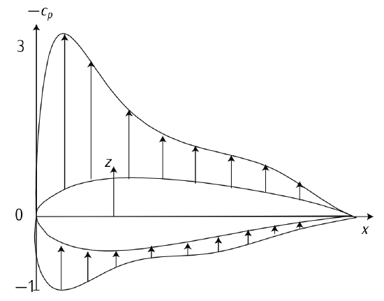
Figure 3.16. Distribution of Coefficient of Pressures. Adapted from \(F_{\text{RANCHINI}}\) et al. [4]

Figure 3.16 shows a typical distribution of coefficient of pressures over an airfoil. Notice that z-axis shows negative \(c_p\) and the direction of arrows means the sign of \(c_p\). An arrow which exits the airfoil implies \(c_p\) is negative, which means the air current accelerates in that area (airfoil’s extrados) and the pressure decreases (suction). On the other hand, where arrows enter the airfoil there exist overpressure, that is, decelerated current and positive \(c_p\). Notice that if there exist a stagnation point (\(V = 0\)), which is by the way typical, \(c_p = 1\).

The dimensionless coefficients are:

\[c_l = \dfrac{l}{\tfrac{1}{2} \rho_{\infty} u_{\infty}^2 c};\]

\[c_d = \dfrac{d}{\tfrac{1}{2} \rho_{\infty} u_{\infty}^2 c};\]

\[c_m = \dfrac{m}{\tfrac{1}{2} \rho_{\infty} u_{\infty}^2 c^2};\]

The criteria of signs is as follows: for \(c_l\), positive if lift goes upwards; for \(c_d\), positive if drag goes backwards; for \(c_m\), positive if the moment makes the airfcraft pitch up.

The equation that allow \(c_l\) and \(c_m\) to be obtained from the distributions of coefficients of pressure in the extrados, \(c_{pe} (x)\), and the intrados, \(c_{pe} (x)\), are:

\[c_l = \dfrac{1}{c} \int_{x_{le}}^{x_{te}} (c_{pi} (x) - c_{pe} (x)) dx = \dfrac{1}{c} \int_{x_{le}}^{x_{te}} c_l (x) dx,\]

\[\begin{array} {rcl} {c_m} & = & {\dfrac{1}{c^2} \int_{x_{le}}^{x_{te}} (x_0 - x) (c_{pi} (x) - c_{pe} (x)) dx = \ ...} \\ {...} & = & {\dfrac{1}{c^2} \int_{x_{le}}^{x_{te}} (x_0 - x) c_l (x) dx.} \end{array}\]

If \(x_0\) is chosen so that the moment is null, \(x_0\) will coincide with the center of pressures of the airfoil (also referred to as aerodynamic center), \(x_{cp}\), which is the point of application of the vector lift:

\[x_{cp} = \dfrac{\int_{x_{le}}^{x_{te}} x c_l (x) dx}{\int_{x_{le}}^{x_{te}} c_l (x) dx}.\]

Notice that in the case of a wing or a full aircraft, lift and drag forces have unities of force [N], and the pitch torque has unities of momentum [Nm]. To represent them it is common agreement to use \(L, D\), and \(M\). In the case of airfoils, due to its bi-dimensional character, typically one talks about force and momentum per unity of distance. In order to notice the difference, they are represented as \(l, d\), and \(m\).

Characteristic curves

The characteristic curves of an airfoil are expressed as a function of the dimensionless coefficients. These characteristic curves are, given a Mach number, a Reynolds number, and the geometry of the airfoil, as follows:

• The lift curve given by \(c_l (\alpha)\).
• The drag curve, \(c_d (c_l)\), also referred to as polar curve.
• The momentum curve, \(c_m (\alpha)\).

Moreover, there is another typical curve which represents the aerodynamic efficiency as a function of \(c_l\) given \(\text{Re}\) and \(M\). The aerodynamic efficiency is \(E = \tfrac{c_l}{c_d} (E = \tfrac{L}{D})\), and measures the ratio between lift generated and drag generated. The designer aims at maximizing this ratio.

Lets focus on the curve of lift. Typically this curve presents a linear zone, which can be approximated by:

\[c_l (\alpha) = c_{l0} + c_{l\alpha} \alpha = c_{l \alpha} (\alpha - \alpha_0),\]

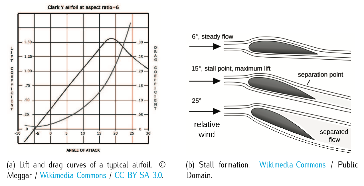
Figure 3.17: Lift and drag characteristic curves.

where \(c_{l \alpha} = d c_l /d \alpha\) is the slope of the lift curve, \(c_{l0}\) is the value of \(c_l\) for \(\alpha = 0\) and \(\alpha_0\) is the value of \(\alpha\) for \(c_l = 0\). The linear theory of thin airfoils in incompressible regime gives a value to \(c_{l \alpha} = 2\pi\), while \(c_{l0}\), which depends on the airfoil’s camber, is null for symmetric airfoils. There is an angle of attack, referred to as stall angle, at which this linear behavior does not hold anymore. At this point the curve presents a maximum. One this point is past lift decreases dramatically. This effect is due to the boundary layer dropping of the airfoil when we increase too much the angle of attack, reducing dramatically lift and increasing drag due to pressure effects. Figure 3.17.b illustrates it.

The drag polar can be approximated (under the same hypothesis of incompressible flow) to a parabolic curve of the form:

\[c_d (c_l) = c_{d_0} + c_{d_i} c_l^2,\]

where \(c_{d_0}\) is the parasite drag coefficient (the one that exist when \(c_l = 0\)) and \(c_{d_i}\) is the induced coefficient (drag induced by lift). This curve is referred to as parabolic drag polar.

The momentum curve can be approximately constant (under the same hypothesis of incompressible flow) if one choses adequately the point \(x_0\). This point is the aerodynamic center of the airfoil. Under incompressible regime, this point is near \(0.25c\).

Lift and drag curves are illustrated in Figure 3.17.a for a typical airfoil.