6.1.1: Propeller propulsion equations

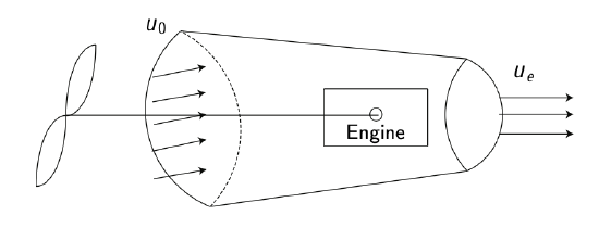
Figure 6.1: Propeller schematic.

A schematic of a propeller propulsion system is shown in Figure 6.1. As the reader would notice, this illustration has strong similarities with the continuity equation illustrated in Figure 3.3. The thrust force is generated due to the change in velocity as the air moves across the propeller between the inlet (0) and outlet (e). As studied in Chapter 3, the mass flow into the propulsion system (considered as a stream tube) is a constant.

The fundamentals of propelled aircraft flights are based on Newton’s equations of motion and the conservation of energy and momentum:

Attending at conservation of momentum principle, the force or thrust is equal to the mass flow times the difference between the exit and inlet velocities, expressed as:

\[F = \dot{m} \cdot (u_e - u_0),\label{eq6.1.1}\]

where \(u_0\) is the inlet velocity, \(u_e\) is the exit velocity, and \(\dot{m}\) is the the mass flow. The exit velocity is higher than the inlet velocity because the air is accelerated within the propeller.

Attending at the conservation of energy principle for ideal systems, the output power of the propeller is equal to the kinetic energy flow across the propeller. This is expressed as follows:

\[P = \dot{m} \cdot (\dfrac{u_e^2}{2} - \dfrac{u_0^2}{2} = \dfrac{\dot{m}}{2} \cdot (u_e - u_0) \cdot (u_e + u_0).\label{eq6.1.2}\]

where \(P\) denotes propeller power.

As real systems do not behave ideally, the propeller efficiency can be defined as:

\[\eta_{prop} = \dfrac{F \cdot u_0}{P}.\label{eq6.1.3}\]

where \(F \cdot u_0\) is the useful work, and \(P\) refers to the input power, i.e., the power that goes into the engine. In other words, the efficiency \(\eta\) is a ratio between the real output power generated to move the aircraft and the input power demanded by the engine to generate it. In an ideal system \(F \cdot u_0 = P\). In real systems \(F \cdot u_0 < P\) due to, for instance, mechanical losses in transmissions, etc.

Operating with Equation (\(\ref{eq6.1.1}\)) and Equation (\(\ref{eq6.1.2}\)) and substituting in Equation (\(\ref{eq6.1.3}\)) it yields:

\[\eta_{prop} = \dfrac{2 \cdot u_0}{u_e + u_0}.\]

In order to obtain a high efficiency (\(\eta_{prop} \sim 1\)), one wants to have \(u_e\) as close as possible to \(u_0\). However, looking at Equation (\(\ref{eq6.1.1}\)), at very close values for input and input velocities, one would need a much larger mass flow to achieve a desired thrust. Therefore, there are find a compromise. Rewriting Equation (\(\ref{eq6.1.1}\)) as:

\[\dfrac{F}{\dot{m} u_0} = \dfrac{u_e}{u_0} - 1,\]

leads to a relation for propulsive efficiency. Notice that, if \(u_e = u_0\), there is no thrust. For higher values of thrust, the efficiency drops dramatically.

Besides the propeller efficiency, other effects contribute to decrease the efficiency of the system. This is the case of the thermal effects in the engine. The thermal efficiency can be defined as:

\[\eta_t = \dfrac{P}{\dot{m}_f \cdot Q},\]

where \(P\) is power, \(\dot{m} f\) is the mass flow of fuel, and \(Q\) is the characteristic heating value of the fuel. 

Finally, the overall efficiency can be defined combining both as follows:

\[\eta_{overall} = \eta_t \cdot \eta_{prop} = \dfrac{F \cdot u_0}{\dot{m}_f \cdot Q}.\]