11.3.1: Autonomous systems

Using only autonomous navigation systems, the most advanced navigation technique to be used is dead reckoning. As shown in Section 11.1, the dead reckoning consist in predicting the future position of the aircraft based on the current position, velocity, and course. Obviously, a reference (or initial) position of the aircraft must be known. In order to determine this reference position, different means can be utilized, e.g., observing a point near the aircraft which position is known (very rudimentary), the observation of celestial bodies (also rudimentary), or the use of the so-called autonomous systems, which are also able to determine the velocity and course of the aircraft.

The two principal autonomous systems are:

• The Doppler radar.
• The Inertial Navigation System (INS).

Doppler radar: A Doppler radar is a specific radar that makes use of the Doppler effect to calculate the velocity of a moving object at some distance. It does so by beaming a microwave signal towards the target, e.g., a flying aircraft, and listening its reflection. Once the reflection has been listened, it is treated analyzing how the frequency of the signal has been modified by the object’s motion. This variation gives direct and highly accurate measurements of the radial component of a target’s velocity relative to the radar.

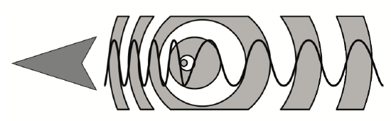
Figure 11.3: Doppler effect: change of wavelength caused by motion of the source. © User:Tkarcher / Wikimedia Commons / CC-BY-SA-3.0.

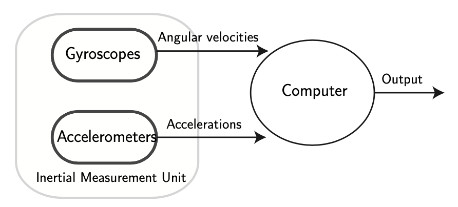
Figure 11.4: Scheme of an Inertial Navigation System (INS). The output refers to position, attitude, and velocity.

Inertial navigation system (INS): An inertial navigation system (INS) includes at least a computer and a platform or module containing accelerometers, gyroscopes, or other motion-sensing devices. The later is referred to as Inertial Measurement Unit (IMU). The computer performs the navigation calculations. The INS is initially provided with its position and velocity from another source (a human operator, a GPS satellite receiver, etc.), and thereafter computes its own updated position and velocity by integrating information received from the motion sensors. Figure 11.4 illustrates it schematically. The advantage of an INS is that it requires no external references in order to determine its position, orientation, or velocity once it has been initialized. On the contrary, the precision is limited, specially for long distances. There are two fundamental inertial navigation systems:

• stable platform systems (aligned with the global reference frame)
• and strap-down systems (aligned with the body frame).

Gyroscopes measure the angular velocity of the aircraft in the inertial reference frame (for instance, the earth-based reference frame). By using the original orientation of the aircraft in the inertial reference frame as the initial condition and integrating the angular velocity, the aircraft’s orientation (attitude) can be known.

Accelerometers measure the linear acceleration of the aircraft, but in directions that can only be measured relative to the moving system (since the accelerometers are attached to the aircraft and rotate with it, but are not aware of their own orientation). Based on this information alone, it is known how the aircraft is accelerating relative to itself, i.e., in a non-inertial reference frame such as the wind reference frame, that is, whether it is accelerating forward, backward, left, right, upwards, or downwards measured relative to the aircraft, but not the direction (attitude) relative to the Earth. The attitude will be an input provided by the gyroscopes.

By tracking both the angular velocity of the aircraft and the linear acceleration of the aircraft measured relative to itself, it is possible to determine the linear acceleration of the aircraft in the inertial reference frame. Performing integration on the inertial accelerations (using the original velocity as the initial conditions) using the correct kinematic equations yields the inertial velocities of the system, and integration again (using the original position as the initial condition) yields the inertial position. These calculations are out of the scope of this course since one needs to take into account relative movement, which is to be studied in advance courses of mechanics. However, some insight is given in Chapter 7 and Appendix A. Two exercises (see Exercises 11.1-11.2) have been proposed for interested readers.

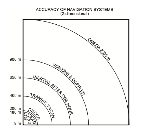
Figure 11.5: Accuracy of navigation systems in 2d. © Johannes Rössel / Wikimedia Commons / CC-BY-SA-3.0

Errors in the inertial navigation system: All inertial navigation systems suffer from integration drift: small errors in the measurement of acceleration and angular velocity are integrated into progressively larger errors in velocity, which are compounded into still greater errors in position. Since the new position is calculated from the previous calculated position and the measured acceleration and angular velocity, these errors are cumulative and increase at a rate roughly proportional to the time since the initial position was input. Therefore the position must be periodically corrected by input from some other type of navigation system. The inaccuracy of a good-quality navigational system is normally less than 0.6 nautical miles per hour in position and on the order of tenths of a degree per hour in orientation. Figure 11.5 illustrates it in relation with other on-autonomous navigation systems (to be studied in what follows).

Accordingly, inertial navigation is usually supplemented with other navigation systems (typically non-autonomous systems), providing a higher degree of accuracy. The idea is that the position (in general, the state of the aircraft) is measured with some sensor, e.g., the GPS, and then, using filtering techniques (Kalman filtering, for instance), estimate the position based on a weighted sum of both measured position and predicted position (the one resulting from inertial navigation). The weighting factors are related to the magnitude of the errors in both measured and predicted position. By properly combining both sources the errors in position and velocity are nearly stable over time. The equation of the Kalman filter are not covered in this course and will be studied in more advanced courses.