
2.1: Basic Microcontroller Use for Measurement and Control
- Page ID
- 46842

Yeyin Shi
Department of Biological Systems Engineering, University of Nebraska-Lincoln, Lincoln, Nebraska, USA
Guangjun Qiu
College of Engineering, South China Agricultural University, Guangzhou, Guangdong, China
Ning Wang
Department of Biosystems and Agricultural Engineering, Oklahoma State University, Stillwater, Oklahoma, USA
Introduction
Measurement and control systems are widely used in biosystems engineering. They are ubiquitous and indispensable in the digital age, being used to collect data (measure) and to automate actions (control). For example, weather stations measure temperature, precipitation, wind, and other environmental parameters. The data can be manually interpreted for better farm management decisions, such as flow rate and pressure regulation for field irrigation. Measurement and control systems are also part of the foundation of the latest internet of things (IoT) technology, in which devices can be remotely monitored and controlled over the internet.
A key component of a measurement and control system is the microcontroller. All biosystems engineers are required to have a basic understanding of what microcontrollers are, how they work, and how to use them for measurement and control. This chapter introduces the concepts and applications of microcontrollers illustrated with a simple project.
Concepts
Measurement and Control Systems
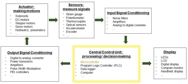
Let’s talk about measurement and control systems first. As shown in Figure 2.1.1, signals can be generated by mechanical actuators and measured by sensors, for example, the voltage signal from a flow rate sensor. The signal is then input to a central control unit, such as a microcontroller, for signal processing, analysis, and decision making. For example, to see if the flow rate is in the desired range or not. Finally, the microcontroller outputs a signal to control the actuator, e.g., adjust the valve opening, and/or at the same time display the system status to users. Then the actuator is measured again. This forms an endless loop that runs continuously until interrupted by the user or time out. If we view the system from the signal’s point of view, the signal generated by the actuators and measured by the sensors are usually analog signals which are continuous and infinite. They are often pre-processed to be amplified, filtered, or converted to a discrete and finite digital format in order to be processed by the central control unit. If the actuator only accepts analog signals, the output signal to control the actuator from the central control unit needs to be converted back to the analog format. As you can tell, the central control unit plays a critical role in the measurement and control loop. Microcontroller is one of the most commonly used central control units. We will focus on microcontrollers in the rest of the chapter.
Microcontrollers
A microcontroller is a type of computer. A computer is usually thought of as a general-purpose device configured as a desktop computer (personal computer; PC or workstation), laptop, or server. The “invisible” type of computer that is widely used in industry and our daily life is the microcontroller. A microcontroller is a miniature computer, usually built as a single integrated circuit (IC) with limited memory and processing capability. They can be embedded in larger systems to realize complex tasks. For example, an ordinary car can have 25 to 40 electronic control units (ECUs), which are built around microcontrollers. A modern tractor can have a similar number of ECUs with microcontrollers handling power, traction, and implement controls. Environmental control in greenhouses and animal houses, and process control in food plants all rely on microcontrollers. Each microcontroller for these applications has a specific task to measure and control, such as air flow (ventilation, temperature) or internal pressure, or to perform higher-level control of a series of microcontrollers. Understanding the basic components of a microcontroller and how it works will allow us to design a measurement and control system.
A microcontroller mainly consists of a central processing unit (CPU), memory units, and input/output (I/O) hardware (Figure 2.1.2). Different components interact with each other and with external devices through signal paths called buses. Each of these parts will be discussed below.
The CPU is also called a microprocessor. It is the brain of the microcontroller, in charge of the primary computation and system internal control. There are three types of information that the CPU handles: (1) the data, which are the digital values to be computed or sent out; (2) the instructions, which indicate which data are required, what calculations to impose, and where the results are to be stored; and (3) the addresses, which indicate where a data or an instruction comes from or is sent to. An arithmetic logic unit (ALU) within the CPU executes mathematical functions on the data structured as groups of binary digits, or “bits.” The value of a bit is either 0 or 1. The more bits a microcontroller CPU can handle at a time, the faster the CPU can compute. Microcontroller CPUs can often handle 8, 16, or 32 bits at a time.
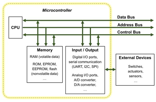
A memory unit (often simply called memory) stores data, addresses, and instructions, which can be retrieved by the CPU during processing. There are generally three types of memory: (1) random-access memory (RAM), which is a volatile memory used to hold the data and programs being executed that can be read from or written to at any time as long as the power is maintained; (2) read-only memory (ROM), which is used for permanent storage of system instructions even when the microcontroller is powered down. Those instructions or data cannot be easily modified after manufacture and are rarely changed during the life of the microcontroller; and (3) erasable-programmable read only memory (EPROM), which is semi-permanent memory that can store instructions that need to be changed occasionally, such as the instructions that implement the specific use of the microcontroller. Firmware is a program usually permanently stored in the ROM or EPROM, which provides for control of the hardware and a standardized operating environment for more complex software programmed by users. The firmware remains unchanged until a system update is required to fix bugs or add features. Originally, EPROMS were erased using ultraviolet light, but more recently the flash memory (electrically erasable programmable read-only memory; EEPROM) has become the norm. The amount of RAM (described in bytes, kilobytes, megabytes, or gigabytes) determines the speed of operation, the amount of data that can be processed and the complexity of the programs that can be implemented.
Digital input and output (I/O) ports connect the microcontroller with external devices using digital signals only. The high and low voltage in the signal correspond to on and off states. Each digital port can be configured as an input port or an output port. The input port is used to read in the status of the external device and the output port is used to send a control instruction to an external device. Most microcontrollers operate over 0 to +5V with limited current because the voltage signal is not used directly, only the binary status. If the voltage and current are to be used to directly drive a device, a relay or voltage digital analog convertor is required between the port and device. Usually digital I/O ports communicate or “talk” with external devices through standard communication protocols, such as serial communication protocols. For example, a microcontroller can use digital I/O pins to form serial communication ports to talk to a general-purpose computer, external memory, or another microcontroller. Common protocols for serial communication are UART (universal asynchronous receiver-transmitter), USB (universal serial bus), I2C (inter-integrated circuit), and SPI (serial peripheral interface). Analog input and output (analog I/O) ports can be connected directly to the microcontroller. Many sensors (e.g., temperature, pressure, strain, rotation) output analog signals and many actuators require an analog signal. The analog ports integrate either an analog to digital (A/D) converter or digital to analog (D/A) converter.
The CPU, memory, and I/O ports are connected through electrical signal conductors known as buses. They serve as the central nervous system of the computer allowing data, addresses, and control signals to be shared among all system components. Each component has its own bus controller. There are three types of buses: the data bus, the address bus, and the control bus. The data bus transfers data to and from the data registers of various system components. The address bus carries the address of a system component that a CPU would like to communicate with or a specific data location in memory that a CPU would like to access. The control bus transmits the operational signal between the CPU and system components such as the read and write signals, system clock signal, and system interrupts.
Finally, clock/counter/timer signals are used in a microcontroller to synchronize operations among components. A clock signal is typically a pulse sequence with a known constant frequency generated by a quartz crystal oscillator. For example, a CPU clock is a high frequency pulse signal used to time and coordinate various activities in the CPU. A system clock can be used to synchronize many system operations such as the input and output data transfer, sampling, or A/D and D/A processes.
Microcontroller Software and Programming
The specific functions of a microcontroller depend on its software or how it is programed. The programs are stored in the memory. Recall that the CPU can only execute binary code, or machine code, and performs low-level operations such as adding a number to a register or moving a register’s value to a memory location. However, it is very difficult to write a program in machine code. Hence, programming languages were developed over the years to make programming convenient. Low-level programming languages, such as assembly language, are the most similar to machine code. They are typically hardware-specific and not interchangeable among different types of microcontrollers. High-level programming languages, such as BASIC, C, or C++, tend to be more generic and can be deployed among different types of microcontrollers with minor modifications.
The programming languages for a specific microcontroller are determined by the microcontroller manufacturer. High-level programming languages are dominant in today’s microcontrollers since they are much easier for learning, interpretation, implementation, and debugging. Programming a microcontroller often requires references to manuals, tutorials, and application notes from manufacturers. Online digital courses and online community-based learning are often good resources as well.
The example presented later in this chapter is a hands-on project using a microcontroller board called Arduino UNO. Arduino is a family of open-source hardware and software, single-board microcontrollers. They are popular and there are many online resources available to help new users develop applications. The microcontrollers are easy to understand and easy to use in real world applications with sensors and actuators (Arduino, 2019). The programming language of the Arduino microcontrollers is based on a language called Processing, which is similar to C or C++ but much simpler (https://processing.org/). The code can be adapted for other microcontrollers. In order to convert codes from a high-level language to the machine code to be executed by a specific CPU, or from one language to another language, a computer program called a compiler is necessary.
Programs can be developed by users in an integrated development environment (IDE), which is a software that runs on a PC or laptop to allow the microcontroller code to be programmed and simulated on the PC or laptop. Most programming errors can be identified and corrected during the simulation. An IDE typically consists of the following components:
- • An editor to program the microcontroller using a relevant high-level programming language such as C, C++, BASIC, or Python.
- • A compiler to convert the high-level language program into low-level assembly language specific to a particular microcontroller.
- • An assembler to convert the assembly language into machine code in binary bit (0 or 1) format.
- • A debugger to error check (also called “debug”) the code, and to test whether the code does what it was intended to do. The debugger typically finds syntax errors, which are statements that cannot be understood and cannot be compiled, and redundant code, which are lines of the program that do nothing. The line number or location of the error is shown by the debugger to help fix problems. The programmer can also add error testing components when writing the code to use the debugger to help confirm the program does what was originally intended.
- • A software emulator to test the program on the PC or laptop before testing on hardware.
Not all components listed above are always presented to the user in an IDE, but they always exist. For the development of some systems, a hardware emulator might also be available. This will consist of a printed circuit board connected to the PC or laptop by ribbon cable joining I/O ports. The emulator can be used to load and run a program for testing before the microcontroller is embedded on a live measurement or control system.
Designing a Microcontroller-Based Measurement and Control System
The following workflow can help us design and build a microcontroller-based measurement and control system.
Step 1. Understand the problem and develop design objectives of the measurement and control system with the end-users. Useful questions to ask include:
- • What should be the functions of the system? For example, a system is needed to regulate the room temperature of a confined animal housing facility within an optimal range.
- • Where or in what environment does the measurement or control occur? For example, is it an indoor or outdoor application? Is the operation in a very high or low temperature, a very dusty, muddy, or noisy environment? Is there anything special to be considered for that application?
- • Are there already sensors or actuators existing as parts of the system or do appropriate ones need to be identified? For example, are there already thermistors installed to measure the room temperature, or are there fans or heaters installed?
- • How frequently and how fast should things be measured or controlled? For example, it may be fine to check and regulate a room temperature every 10 seconds for a greenhouse; however, the flow rate and pressure of a variable-rate sprayer running at 5 meters per second (about 12 miles per hour) in the field need to be monitored and controlled at least every second.
- • How much precision does the measurement and control need? For example, is a precision of a Celsius degree enough or does the application need sub-Celsius level precision?
Step 2. Identify the appropriate sensors and/or actuators if needed for the desired objectives developed in the previous step.
Step 3. Understand the input and output signals for the sensors and actuators by reading their specifications.
- • How many inputs and outputs are necessary for the system functions?
- • For each signal, is it a voltage or current signal? Is it a digital or analog signal?
- • What is the range of each signal?
- • What is the frequency of each signal?
Step 4. Select a microcontroller according to the desired system objective, the output signals from the sensors, and the input signals required by the actuators. Read the technical specifications of the microcontroller carefully. Be sure that:
- • the number and types of I/O ports are compatible with the output and input signals of the sensors and actuators;
- • the CPU speed and memory size are enough for the desired objectives;
- • there are no missing components between the microcontroller, the sensors, and actuators such as converters or adapters, and if there are any, identify them; and
- • the programming language(s) of the microcontroller is appropriate for the users.
Step 5. Build a prototype of the system with the selected sensors, actuators, and microcontroller. This step typically includes the physical wiring of the hardware components. If preferred, a virtual system can be built and tested in an emulator software to debug problems before building and testing with the physical hardware to avoid unnecessary hardware damage.
Step 6. Program the microcontroller. Develop a program with all required functions. Load it to the microcontroller and debug with the system. All code should be properly commented to make the program readable by other users later.
Step 7. Deploy and debug the system under the targeted working environment with permanent hardware connections until everything works as expected.
Step 8. Document the system including, for example, specifications, a wiring diagram, and a user’s manual.
Applications
Microcontroller-based measurement and control systems are commonly used in agricultural and biological applications. For example, a field tractor has many microcontrollers, each working with different mechanical modules to realize specific functions such as monitoring and maintaining engine temperature and speed, receiving GPS signals for navigation and precise control of implements for planting, spraying, and tillage. A linear or center pivot irrigation system uses microcontrollers to ensure flow rate, nozzle pressure, and spray pattern are all correct to optimize water use efficiency. Animal logging systems use microcontrollers to manage the reading of ear tags when the animals pass a weighing station or need to be presented with feed. A food processing plant uses microcontroller systems to monitor and regulate processes requiring specific throughput, pressure, temperature, speed, and other environmental factors. A greenhouse control system for vegetable production will be used to illustrate a practical application of microcontrollers.
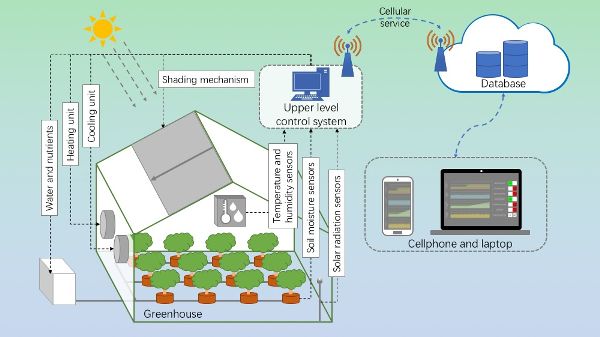
Modern greenhouse systems are designed to provide an optimal environment to efficiently grow plants with minimal human intervention. With advanced electronic, computer, automation, and networking technologies, modern greenhouse systems provide real-time monitoring as well as automatic and remote control by implementing a combination of PC communication, data handling, and storage, with microcontrollers each used to manage a specific task (Figure 2.1.3). The specific tasks address the plants’ need for correct air composition (oxygen and carbon dioxide), water (to ensure transpiration is optimized to drive nutrient uptake and heat dispersion), nutrients (to maximize yield), light (to drive photosynthesis), temperature (photosynthesis is maximized at a specific temperature for each type of plant, usually around 25°C) and, in some cases, humidity (to help regulate pests and diseases as well as photosynthesis). In a modern greenhouse, photosynthesis, nutrient and water supplies, and temperature are closely monitored and controlled using multiple sensors and microcontrollers.
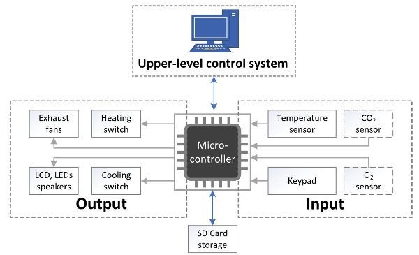
As shown in Figure 2.1.3, the overall control of the greenhouse environment is divided into two levels. The upper-level control system (Figure 2.1.4) integrates an array of lower-level microcontrollers, each responsible for specific tasks in specific parts of the greenhouse, i.e., there may be multiple microcontrollers regulating light and shade in a very large greenhouse.
At the lower level, microcontrollers may work in sub-systems or independently. Each microcontroller has its own suite of sensors providing inputs, actuators controlled by outputs, an SD (secure digital) card as a local data storage unit, and a CPU to run a program to deliver functionality. Each program implements its rules or decisions independently but communicates with the upper-level control system to receive time-specific commands and to transmit data and status updates. Some sub-systems may be examined in more detail and more frequently.
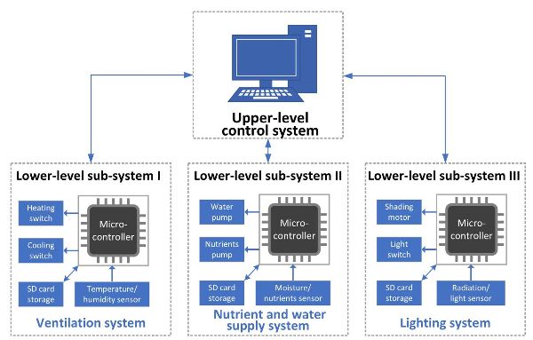
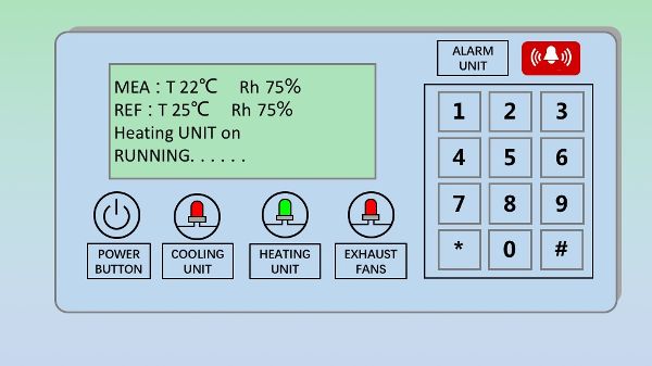
The ventilation sub-system is designed to maintain the temperature and humidity required for optimal plant growth inside the greenhouse. A schematic of a typical example (Figure 2.1.5) shows the sub-system structure. Multiple temperature and humidity sensors are installed at various locations in the greenhouse and connected to the inputs of a microcontroller. Target temperature and humidity values can be input using a keypad connected to the microcontroller (Figure 2.1.6) or set by the upper-level control system. Target values are also called “control set points” or simply “set points.” They are the values the program is designed to maintain for the greenhouse. The microcontroller’s function is to compare the measured temperature and humidity with the set point values to make a decision and adjust internal temperature. If a change is needed, the microcontroller controls actuators to turn on a heating device to raise the temperature (if temperature is below set point) or a cooling system fan (if temperature is above set point) to bring the greenhouse to the desired temperature and humidity.
The control panel in a typical ventilation system is shown in Figure 2.1.6. Here a green light indicates that the heating unit is running, while the red lights indicate that both the cooling unit and exhaust fans are off. The LCD displays the measured temperature and relative humidity inside the greenhouse (first line of text), the set point temperature and humidity values (second line of text), the active components (third line of text) and system status (fourth line of text). As the measured temperature is cooler than the set point, the heating unit has been turned on to increase the temperature from 22°C to 25°C. When the measured temperature reaches 25°C, the heating unit will be switched off. It is also possible to program alarms to alert an operator when any of the measured values exceed critical set points.
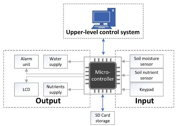
The nutrient and water supply sub-system (Figure 2.1.7) provides plants with water and nutrients at the right time and the right amounts. It is possible to program a preset schedule and preset values or to respond to sensors in the growing medium (soil, peat, etc.). As in the temperature and humidity sub-system, the user can manually input set point values, or the values can be received from the upper-level system. Ideally, multiple sensors are used to measure soil moisture and nutrient levels in the root zone at various locations in the greenhouse. The readings of the sensors are interpreted by the microcontroller. When measured water or nutrient availability drops below a threshold, the microcontroller controls an actuator to release more water and/or nutrients.
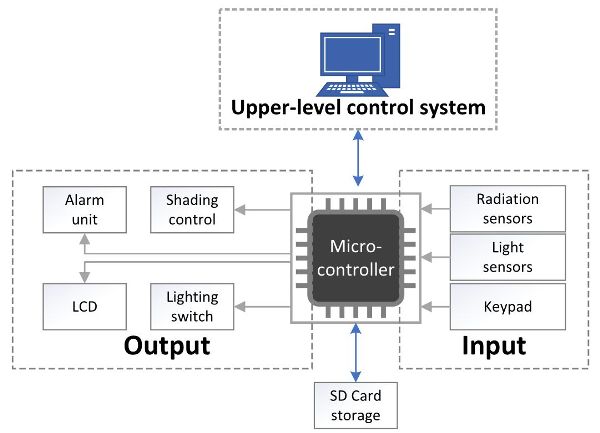
The lighting sub-system (Figure 2.1.8) is designed to replace or supplement solar radiation provided to the plants for photosynthesis. Solar radiation and light sensors are installed in the greenhouse. The microcontroller reads data from these sensors and compares them with set points. If the measured value is too high, the microcontroller actuates a shading mechanism to cover the roof area. If the measured value is too low, the microcontroller activates the shading mechanism to remove all shading and, if necessary, turns on supplemental light units.
The upper-level control system is usually built on a PC or a server, which provides overall control through an integration of the subsystems. All of the sub-systems are connected to the central control computer through serial or wireless communication, such as an RS-232 port, Bluetooth, or Ethernet. The central control computer collects the data from all of the subsystems for processing analysis and record keeping. The upper-level control system can make optimal control decisions based on the data from all subsystems. It also provides an interface for the operator to manage the whole system, if needed. The central control computer also collects all data from all sensors and actuators to populate a database representing the control history of the greenhouse. This can be used to understand failure and, once sufficient data are collected, to implement machine learning algorithms, if required.
This greenhouse application is a simplified example of a practical complex control system. Animal housing and other environmental control problems are of similar complexity. Modern agricultural machinery and food processing plants can be significantly more complex to understand and control. However, the principle of designing a hierarchical system with local automation managed by a central controller is very similar. Machine learning and artificial intelligence are now being used to achieve precise and accurate controls in many applications. Their control algorithms and strategies can be implemented on the upper-level control system, and the control decisions can be sent to the lower-level subsystems to implement the control functions.
Example
Example \(\PageIndex{1}\)
Example 1: Low-Cost Temperature Measurement and Control System
Problem:
A farmer wants to develop a low-cost measurement and control system to help address heat and cold stresses in confined livestock production. Specifically, the farmer wants to maintain the optimal indoor temperature of 18° to 20°C for a growing-finishing pig barn. A heating/cooling system needs to be activated if the temperature is lower or higher than the optimal range. The aim is to make a simple indicator to alert the stock handlers when the temperature is out of the target range, so that they can take action. (Automatic heating and cooling control is not required here.) Design and build a microcontroller-based measurement and control system to meet the specified requirements.
Solution
Complete the recommended steps discussed above.
Step 1. Understand the problem.
- • Functions—We need a system to monitor the ambient temperature and make alerts when the temperature is out of the 18° to 20°C range. The alert needs to indicate whether it is too cold or too hot, and the size of the deviation from that range.
- • Environment—As a growing-finishing pig barn can be noisy, we will use a visual indicator as an alert rather than a sound alert.
- • Existing sensors or actuators—For this example, assume that heating and cooling mechanisms have been installed in the barn. We just need to automate the temperature monitoring and decision-making process.
- • Frequency—The temperature in a growing-finishing pig barn usually does not change rapidly. In this example, let’s assume the caretakers require the temperature to be monitored every second.
- • Precision—In this project, let’s set the requirements for the precision at one degree Celsius for the temperature control.
Step 2. Identify the appropriate sensors and/or actuators.
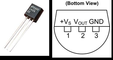
The sensor that will be used in this example to measure temperature is the Texas Instruments LM35. It is one of the most widely used, low-cost temperature sensors in measurement and control systems in industry. Its output voltage is linearly proportional temperature, so the relationship between the sensor output and the temperature is straightforward.
We will use an RGB LED to light in different colors and blink at different rates to indicate the temperature and make alerts. This type of LED is a combination of a red LED, a green LED, and a blue LED in one package. By adjusting the intensity of each LED, a series of colors can be made. In this example, we will light the LED in blue when a temperature is lower than the optimal range, in green when the temperature is within the optimal range, and in red when the temperature is higher than the optimal range. In addition, the further the temperature has deviated from the optimal range, the faster the LED will blink. In this way, we alert the caretakers that a heating or cooling action needs to be taken and how urgent the situation is.
Step 3. Understand the input and output signals.
The LM35 series are precision integrated circuit temperature sensors with an output voltage linearly proportional to the Celsius (C) temperature (LM35 datasheet; http://www.ti.com/lit/ds/symlink/lm35.pdf). There are three pins in the LP package of the sensors as shown in Figure 2.1.9. A package is a way that a block of semiconductors is encapsulated in a metal, plastic, glass, or ceramic casing.
- • The +VS pin is the positive power supply pin with voltage between 4V and 20V (in this project, we use +5V);
- • The VOUT pin is the temperature sensor analog output of no more than 6V (5V for this project);
- • The GND pin is the device ground pin to be connected to the power supply negative terminal.
The accuracy specifications of the LM35 temperature sensor are given with respect to a simple linear transfer function:
\[ V_{out} =10 \text{mV}\ ^{\circ}C \times T \]
where VOUT is the temperature sensor output voltage in millivolts (mV) and T is the temperature in °C.
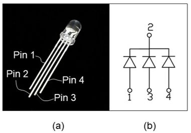
In an RGB LED, each of the three single-color LEDs has two leads, the anode (or positive pin) where the current flows in and the cathode (or negative pin) where the current flows out. There are two types of RGB LEDs: common anode and common cathode. Assume we use the common cathode RGB LED as show in Figure 2.1.10 but the other type would also work. The common cathode (–) pin 2 will connect to the ground. The anode (+) pins 1, 3, and 4 will connect to the digital output pins of the microcontroller.
Step 4. Select a microcontroller.
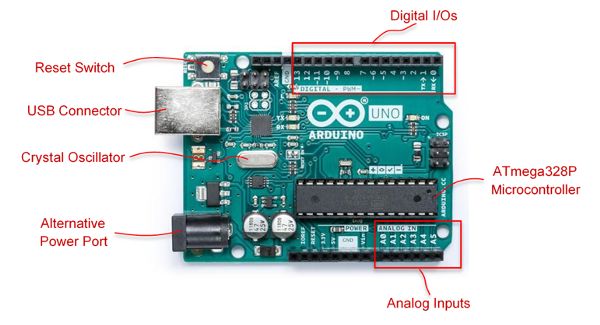
There are many general-purpose microcontrollers available commercially, such as the Microchip PIC, Parallax BASIC Stamp 2, ARM, and Arduino (Arduino, 2019). In this example, we will select an Arduino UNO microcontroller board based on the ATmega328P microcontroller (https://store.arduino.cc/usa/arduino-uno-rev3) (Figure 2.1.11). The microcontroller has three types of memory: a 2KB RAM where the program creates and manipulates variables when it runs; a 1KB EEPROM where long-term information such as the firmware of the microcontroller is stored, and 32KB flash memory that can be used to store the programs you developed. The flash memory and EEPROM memory are non-volatile, which means the information persists after the power is turned off. The RAM is volatile, and the information will be lost when the power is removed. There are 14 digital I/O pins and 6 analog input pins on the Arduino UNO board. There is a 16 MHz quartz crystal oscillator. ATmega-based boards, including the Arduino UNO, take about 100 microseconds (0.0001 s) to read an analog input. So, the maximum reading rate is about 10,000 times a second, which is more than enough for our desired sampling frequency of every second. The board runs at 5 V. It can be powered by a USB cable, an AC-to-DC adapter, or a battery. If an USB cable is used, it also serves for loading, running, and debugging the program developed in the Arduino IDE. The Arduino UNO microcontroller is compatible with the LM35 temperature sensor and the desired control objectives of this project.
Step 5. Build a prototype.
The materials you need to build the system are:
- • Arduino UNO board × 1
- • Breadboard × 1
- • Temperature sensor LM35 × 1
- • RGB LED × 1
- • 220 Ω resistor × 3
- • Jumper wires
Figure 2.1.12 shows the hardware wiring.
- • Pin 1 of the temperature sensor goes to the +5V power supply on the Arduino UNO board;
- • Pin 2 of the temperature sensor goes to the analog pin A0 on the Arduino UNO board;
- • Pin 3 of the temperature sensor goes to one of the ground pin GND on the Arduino UNO board;
- • Digital I/O pin 2 on the Arduino UNO board connects with pin 4 (the blue LED) of the RGB LED through a 220 Ω resistor;
- • Digital I/O pin 3 on the Arduino UNO board connects with pin 3 (the green LED) of the RGB LED through a 220 Ω resistor;
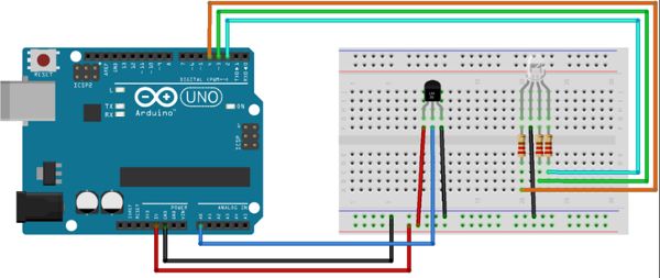
- • Digital I/O pin 4 on the Arduino UNO board connects with pin 1 (the red LED) of the RGB LED through a 220 Ω resistor; and
- • Pin 2 (cathode) of the RGB LED connects to the ground pin GND on the Arduino UNO board.
An electronics breadboard (Figure 2.1.13) is used to create a prototyping circuit without soldering. This is a great way to test a circuit. Each plastic hole on the breadboard has a metal clip where the bare end of a jumper wire can be secured. Columns of clips are marked as +, −, and a to j; and rows of clips are marked as 1 to 30. All clips on each one of the four power rails on the sides are connected. There are typically five connected clips on each terminal strip.
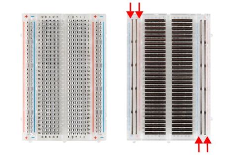
(a) (b)
Figure \(\PageIndex{13}\): A breadboard: (a) front view (b) back view with the adhesive back removed to expose the bottom of the four vertical power rails on the sides (indicated with arrows) and the terminal strips in the middle. (Picture from Sparkfun, https://learn.sparkfun.com/tutorials/how-to-use-a-breadboard/all).
Step 6. Program the microcontroller.
The next step is to develop a program that runs on the microcontroller. As we mentioned earlier, programs are developed in IDE that runs either on a PC, a laptop, or a cloud-based online platform. Arduino has its own IDE. There are two ways to access it. The Arduino Web Editor (https://create.arduino.cc/editor/) is the online version that enables developers to write code, access tutorials, configure boards, and share projects. It works within a web browser so there is no need to install the IDE locally; however, a reliable internet connection is required. The more conventional way is to download and install the Arduino IDE locally on a computer (https://www.arduino.cc/en/main/software). It has different versions that can run on Windows, Mac OS X, and Linux operating systems. For this project, we will use the conventional IDE installed on a PC running Windows. The way the IDE is set up and operates is similar between the conventional one and the web-based one. You are encouraged to try both and find the one that works best for you.
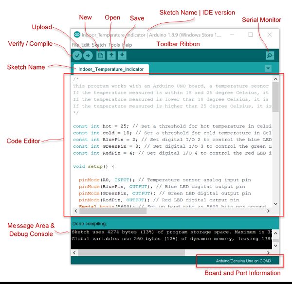
Follow the steps on the link https://www.arduino.cc/en/Main/Software#download to download and install the Arduino IDE with the right version for your operating system. Open the IDE. It contains a few major components as shown in Figure 2.1.14: a Code Editor to write text code, a Message Area and Debug Console to show compile information and error messages, a Toolbar Ribbon with buttons for common functions, and a series of menus.
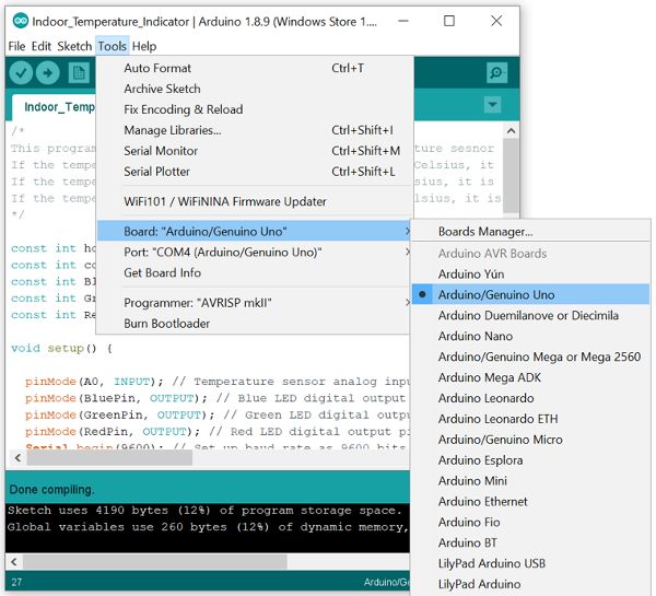
Make sure that you disconnect the plug-ins of all the wires and pins the first time you power on the Arduino board either with a USB cable or a DC power port. It is a good habit to never connect or disconnect any wires or pins when the board is power on. Connect the Arduino UNO board and your PC or laptop using the USB cable. Under “Tools” in the main menu (Figure 2.1.15) of the Arduino IDE, select the right board from the drop-down menu of “Board:” and the right COM port from the drop-down menu of “Port:” (which is the communication port the USB is using). Then disconnect the USB cable from the Arduino UNO board.
Now let’s start coding in the Code Editor of the IDE. An Arduino board runs with a programming language called Processing, which is similar to C or C++ but much simpler (https://processing.org/). We will not cover the details about the programming syntax here; however, we will explain some of them along with the programming structure and logic. At the same time, you are encouraged to go to the websites of Arduino and the Processing language to learn more details about the syntax of Arduino programming.
Arduino programs have a minimum of 2 blocks—a setup block and an execution loop block. Each block has a set of statements enclosed in a pair of curly braces:
/*
Setup Block
*/
void setup() { // Opening brace here
Statements 1; // Semicolon after every statement
Statements 2;
...
Statements n;
} // Closing brace here
/*
Execution Loop Block
*/
void loop() { // Opening brace here
Statements 1; // Semicolon after every statement
Statements 2;
...
Statements n;
} // Closing brace here
There must be a semicolon (;) after every statement to indicate the finish of a statement; otherwise, the IDE will return an error during compiling. Statements after “//” in a line or multiple lines of statements between the pair of “/*” and “*/” are comments. Comments will not be compiled and executed, but they are important to help the readers understand the code.
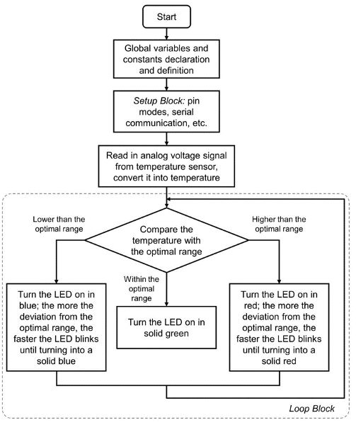
The program logic flowchart is shown in Figure 2.1.16. To better understand the code, we will separate the code into a few parts according to the logic flowchart. Each part will have its associated code shown in a grey box with explanations. You can copy and paste them into the Code Editor in the Arduino IDE. When writing the codes, be sure to save them frequently.
Program Part 1—Introductive Comments
Here we use multiple lines of statements to summarize the general purpose and function of the code.
/*
This program works with an Arduino UNO board, a temperature sensor and an RGB LED to measure and indicate the ambient temperature.
If the temperature measured is within 18 and 20 degree Celsius, it is considered as optimal temperature and the LED is lit in green color.
If the temperature measured is lower than 18 degree Celsius, it is considered as cold and the LED is lit in blue color and blinks. The colder the temperature, the faster the LED blinks.
If the temperature measured is higher than 20 degree Celsius, it is considered as hot and the LED is lit in red color and blinks. The hotter the temperature, the faster the LED blinks.
*/
Program Part 2—Declarations of Global Variables and Constants
In this part of the program, we define a few variables and constants that will be used later for the entire program, including the upper and lower thresholds of the optimal temperature range and the numbers of the digital pins for the red, green, and blue LEDs inside the RGB LED, respectively. For example, the first statement here, “const int hot = 20” means that a constant (“const”) integer (“int”) called “hot” is created and assigned to the value of “20” which is the upper limit of the optimal temperature range. The third statement here, “const int BluePin = 2,” means that a constant (“const”) integer (“int”) called “BluePin” is created and assigned to the value of “2” which will be used later in the setup block of the program to set digital pin 2 as the output pin to control the blue LED.
const int hot = 20; // Set a threshold for hot temperature in Celsius
const int cold = 18; // Set a threshold for cold temperature in Celsius
const int BluePin = 2; // Set digital I/O 2 to control the blue LED in the RGB LED
const int GreenPin = 3; // Set digital I/O 3 to control the green LED in the RGB LED
const int RedPin = 4; // Set digital I/O 4 to control the red LED in the RGB LED
Program Part 3—Setup Block
As mentioned earlier, the setup block must exist even if there are no statements to execute. It is executed only once before the microcontroller executes the loop block repeatedly. Usually the setup block includes the initialization of the pin modes and the setup and start of serial communication between the microcontroller and the PC or laptop where the IDE runs. In this example, we set the analog pin A0 as the input of the temperature sensor measurements, digital pins defined earlier in Part 2 of the code as output pins to control the RGB LED, and start the serial communication with a typical communication speed (9600 bits per second) so that everything is ready for the microcontroller to execute the loop block.
void setup() {
pinMode(A0, INPUT); // Temperature sensor analog input pin
pinMode(BluePin, OUTPUT); // Blue LED digital output pin
pinMode(GreenPin, OUTPUT); // Green LED digital output pin
pinMode(RedPin, OUTPUT); // Red LED digital output pin
Serial.begin(9600); // Set up baud rate as 9600 bits per second
}
Program Part 4—Execution Loop Block
The loop part of the program is what the microcontroller runs repeatedly unless the power of the microcontroller is turned off.
Program Part 4.1—Start the loop and read in the analog input from the temperature sensor:
void loop() {
int sensor = analogRead(A0); // Read in the value from the analog pin connected to
// the temperature sensor
float voltage = (sensor / 1023.0) * 5.0; // Convert the value to voltage
float tempC = (voltage – 0.5) * 100; // Convert the voltage to temperature using the
/* scale factor; 0.5 is the deviation of the output voltage versus temperature from the best-fit straight line derived from sensor calibration */
Serial.print(“Temperature: ”);
Serial.print(tempC); // Print the temperature on the Arduino IDE output console
Here you see two types of variables, the integer (“int”) and the float (“float”). For an Arduino UNO, an “int” is 16 bit long and can represent a number ranging from −32,768 to 32,767 (−2^15 to (2^15) − 1). A “float” in Arduino UNO is 32 bit long and can represent a number that has a decimal point, ranging from −3.4028235E+38 to 3.4028235E+38. Here, we define the variable of the temperature measured from the LM35 sensor as a float type so that it can represent a decimal number and is more accurate.
Program Part 4.2—Check if the temperature is lower than the optimal temperature range. If yes, turn on the LED in blue and blink it according to how much the temperature deviated from the optimal range:
if (tempC < cold) { // If the temperature is colder than the optimal temperature range
Serial.println(“It’s cold.”);
// the optimal range
if (temp_dif <= 10) {
/* Calculate LED blink interval in milliseconds based on the temperature deviation from the optimal range; the further the deviation, the faster the LED blinks until turning into a solid blue */
// Blink the LED in blue:
digitalWrite(BluePin, HIGH); // Turn on the blue LED
digitalWrite(GreenPin, LOW); // Turn off the green LED
digitalWrite(RedPin, LOW); // Turn off the red LED
delay(LED_blink_interval); // Keep this status for a certain amount of time in milliseconds
digitalWrite(BluePin, LOW); // Turn off the blue LED
delay(LED_blink_interval); // Keep this status for a certain amount of time in milliseconds
}
else {
digitalWrite(BluePin, HIGH); // Turn off the blue LED
digitalWrite(GreenPin, LOW); // Turn off the green LED
digitalWrite(RedPin, LOW); // Turn on the red LED
}
}
Here, we define an integer variable called “LED_blink_interval” which is inversely proportional to the deviation of the temperature from the optimal range “temp_dif.” A coefficient 4000 is used here to convert the number to something close to 1000. Arduino always measures the time duration in millisecond, so delay(1000) means delay for 1000 millisecond, or 1 second.
Program Part 4.3—Check if the temperature is higher than the optimal temperature range. If yes, turn on the LED in red and blink it according to how much the temperature deviated from the optimal range:
else if (tempC > hot) {
// If the temperature is hotter than the optimal temperature range
Serial.println(“It’s hot.”);
// Calculate how much the temperature deviated from the optimal range
if (temp_dif <= 10) {
/* Calculate LED blink interval in milliseconds based on the temperature
deviation from the optimal range; the further the deviation, the faster the LED blinks until turning into a solid red */
// Blink the LED in red:
digitalWrite(BluePin, LOW); // Turn off the blue LED
digitalWrite(GreenPin, LOW); // Turn off the green LED
digitalWrite(RedPin, HIGH); // Turn on the red LED
delay(LED_blink_interval); // Keep this status for certain time in ms
digitalWrite(RedPin, LOW); // Turn off the red LED
delay(LED_blink_interval); // Keep this status for certain time in ms
}
else {
digitalWrite(BluePin, LOW); // Turn off the blue LED
digitalWrite(GreenPin, LOW); // Turn off the green LED
digitalWrite(RedPin, HIGH); // Turn on the red LED
}
Program Part 4.4—If the temperature is within the optimal range, turn on the LED in green:
else { // Otherwise the temperature should be fine; turn the LED on in solid green
Serial.println(“The temperature is fine.”);
digitalWrite(BluePin, LOW); // Turn off the blue LED
digitalWrite(GreenPin, HIGH); // Turn on the green LED
digitalWrite(RedPin, LOW); // Turn off the red LED
}
delay(10);
}
After the program is written, use the “verify” button in the IDE to compile the code and debug errors if there are any. If the code has been transcribed accurately, there should be no syntax errors or bugs. If the IDE indicates errors, it is necessary to work through each line of code to make sure the program is correct. Be aware that sometimes the real error indicated by the debugger is in the lines before or after the location indicated. Some common errors include missing variable definition, missing braces, wrong spelling for a function, and letter capitalization error. Some other errors, such as the wrong selection of variable type, often cannot be caught during the compile stage, but we can use the “Serial.print” function to print the results or intermediate results on the serial monitor to see if they look reasonable.
Once the program code has no errors, connect the PC or laptop with the Arduino UNO board without any wire or pin plug-ins using the USB cable. Check if the selections for the type of board and port options under “Tools” in the main menu are still right. Use the “upload” button in the IDE to upload the program code to the Arduino board. Disconnect the USB cable from the board, and now plug in all the wires and pins. Re-connect the board and open the “Serial Monitor” from the IDE. The current ambient temperature should display in the serial monitor, and the LED lights color and blink accordingly. If any further errors occur, they will show in the message area at the bottom part of the IDE window. Go back to debugging if this happens. If there are no errors and everything runs correctly, test how the measurement system works by changing the temperature around the sensor to see the corresponding response of the LED color and blinking frequency. This can be done by breathing over the sensor or placing it close to a cup of iced water or in a fridge for a short time. When the room temperature is in the set point range (about 18°C to 20°C) the green LED should be lit. Once the temperature is too high, only the red LED should be lit. When the temperature is too low, only the blue LED should be lit. If this does not work, check that you have created different temperatures by using a laboratory thermometer and then check the program code.
Step 7. Deploy and debug.
Deploy and debug the system under the targeted working environment with permanent hardware connections until everything works as expected.
We leave this step of making the permanent hardware connections for you to complete if interested. In practice, the packaging of the overall system will be designed to accommodate the working environment. The completed final product will be tested extensively for durability and reliability.
Step 8. Document the system.
Write documentation such as system specifications, wiring diagram, and user’s manual for the end users. At this stage, an instruction and safety manual would be written, and, if necessary, the product can be sent for local certification. Now the system you developed is ready to be signed off and handed over to the end users!
Image Credits
Figure 1. Alciatore, D.G., and Histand, M.B. (CC By 4.0). (2012). Main components in a measurement and control system. Introduction to mechatronics and measurement systems. Fourth edition. McGraw Hill.
Figure 2. Alciatore, D.G., and Histand, M.B. (2013). Microcontroller architecture. Adapted from Introduction to mechatronics and measurement systems. Fourth edition. McGraw Hill.
Figure 3. Qiu, G. (CC By 4.0). (2020). A diagram of a modern greenhouse system.
Figure 4. Qiu, G. (CC By 4.0). (2020). The core structure of a greenhouse control system.
Figure 5. Qiu, G. (CC By 4.0). (2020). The schematic of ventilation system.
Figure 6. Qiu, G. (CC By 4.0). (2020). The schematic of the control panel in ventilation system.
Figure 7. Qiu, G. (CC By 4.0). (2020). The nutrient and water supply system.
Figure 8. Qiu, G. (CC By 4.0). (2020). The schematic of lighting system.
Figure 9. Texas Instrument. (2020). Texas Instruments LM35 precision centigrade temperature sensor in LP package (a) and its pin configuration and functions (b). Retrieved from http://www.ti.com/lit/ds/symlink/lm35.pdf
Figure 10. Amazon. (2020). A 5 mm common cathode RGB LED and its pinout. Retrieved from www.amazon.com/Tricolor-Diffused-Multicolor-Electronics-Components/dp/B01C3ZZT8W/ref=sr_1_36?keywords=rgb+led&qid=1574202466&sr=8-36
Figure 11. Arduino. (2020). An Arduino UNO board and some major components. Retrieved from https://store.arduino.cc/usa/arduino-uno-rev3
Figure 12. Shi, Y. (CC By 4.0). (2020). Wiring diagram for setting up the test platform.
Figure 13. Sparkfun. (CC By 4.0). (2020). A breadboard: (a) front view (b) back view with the adhesive back removed to expose the bottom of the four vertical power rails on the sides (indicated with arrows) and the terminal strips in the middle Retrieved from https://learn.sparkfun.com/tutorials/how-to-use-a-breadboard/all
Figure 14. Shi, Y. (CC By 4.0). (2020). The interface and anatomy of Arduino IDE.
Figure 15. Shi, Y. (CC By 4.0). (2020). Select the right board and COM port in Arduino IDE.
Figure 16. Shi, Y. (CC By 4.0). (2020). Program logic flowchart.
References
Alciatore, D. G., and Histand, M. B. 2012. Introduction to mechatronics and measurement systems. 4th ed. McGraw Hill.
Arduino, 2019. https://www.arduino.cc/ Accessed on March 15, 2019.
Bolton, W. 2015. Mechatronics, electronic control systems in mechanical and electrical engineering. 6th ed. Pearson Education Limited.
Carryer, J. E., Ohline, R. M., and Kenny, T.W. 2011. Introduction to mechatronic design. Prentice Hall.
de Silva, C. W. 2010. Mechatronics—A foundation course. CRC Press.
University of Florida. 2019. What makes plants grow? edis.ifas.ufl.edu/pdffiles/4h/4H36000.pdf.