
3.1: Traction
- Page ID
- 46845

Daniel M. Queiroz
Department of Agricultural Engineering
Universidade Federal de Vicosa
Viçosa, Minas Gerais, Brazil
John K. Schueller
Department of Mechanical and Aerospace Engineering
University of Florida
Gainesville, Florida, USA
| Key Terms |
| Mechanics of traction | Traction devices | Tractors |
| Engine power | Transport devices | Pulled implements |
| Tractive force |
Variables
Introduction
Tractors were created to reduce human and animal labor inputs and increase efficiency and productivity in crop production activities (Schueller, 2000). The main use of tractors is to pull implements such as tillage tools, planters, cultivators, and harvesters in the field and, to some extent, on the road (Renius, 2020). To pull implements efficiently, a tractor needs to generate traction between the tires and the soil surface. Traction is the way a vehicle uses force to move over a surface.
Quite early in tractor development, the direct transfer of power from tractors to implements was made possible by using power take-offs (PTOs) that transfer rotary power to implements and machines and by using hydraulic systems to lift and lower implements and to move parts of attached machines. Pulling implements is still the most common use of tractor power. The field capacity of agricultural machines, i.e., the field area that can be covered per unit time, has caused bigger implements to be developed and used. The increased sizes require greater traction from the pulling tractor. More efficient systems to create the tractive force are necessary to provide the large forces necessary to pull those implements.
The efficiency of how tractors convert the power generated by an engine to the power required to pull the implements depends on many variables associated with the tractor and the soil conditions. Traction is especially important in agriculture as field soils are not as firm as the roads used by cars and trucks. This chapter presents the basic principles of traction applied to agricultural machinery.
Outcomes
After reading this chapter, you should be able to:
- • Explain how tractors develop tractive force
- • Describe the effect of some important variables on the tractive force
- • Calculate how much power a tractor can develop when pulling an implement
- • Calculate the power requirements to match tractors to implements
Concepts
Traction and Transport Devices
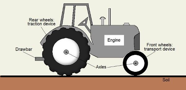
According to the American Society of Agricultural and Biological Engineers (ASABE Standards, 2018), there are two types of surface contact devices associated with the motion of a vehicle: traction devices and transport devices. A traction device receives power from an engine and uses the reactions of forces from the supporting surface to propel the vehicle, while a transport device does not receive power, but is needed to support the vehicle on a surface while the vehicle is moving over that surface. Wheels, tires, and tracks can be traction devices if they are connected to an engine or other power source; if not connected, they are transport devices. The main components of an agricultural tractor are presented in Figure 3.1.1. In this example, the tractor is 2-wheel drive, so the large rear wheels, which receive power from the engine, are the traction devices, and the small front wheels are the transport devices. All wheels would be traction devices if the tractor were 4-wheel drive. The engine is connected to the traction device by the drive train, often consisting of a clutch, transmission, differential, axles, and other components. (The drive train is not discussed in this chapter.) The drawbar is an attachment point through which the tractor can apply pulling force to an implement.
Mechanics of Traction
The simplest way of analyzing the traction produced by a traction device, such as a wheel or track, is to consider friction forces that act at the contact between a traction device and the surface when the system is in equilibrium. For simplification the machine is assumed to be moving at a constant velocity on a non-variable surface (Figure 3.1.2). A traction device (hereafter simplified to the most common implementation as a “wheel”) has two main functions: to support the load acting on the wheel axle (W) and to produce a net tractive force (H). The force W is generally called the dynamic load acting on the wheel. The dynamic load depends on how the weight of the tractor at that point in time is distributed to each wheel. If the system is in equilibrium, the surface reacts to W by applying a vertical reaction force (R) to the wheel. In the contact between the surface and the wheel, a friction force (Ff) is generated. To keep equilibrium in the horizontal direction, the magnitude of the net tractive force H is equal to the magnitude of the friction force Ff. To produce a net tractive force H, the friction force needs to be overcome. This is done by applying a torque (T) to the wheel axle. This torque is proportional to the torque produced by the tractor engine according to the drive train, including the current transmission ratio.
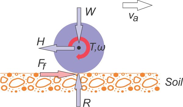
When moving, the wheel (Figure 3.1.2) rotates with a constant angular velocity (ω), and this angular speed is proportional to the engine rotation speed, depending on the gearing ratio in the drive train. The wheel has an actual velocity va, which is equal to the angular velocity multiplied by the wheel’s rolling radius reduced by the slip (as discussed below). In an equilibrium situation, ω and va are constants. The power transferred to the wheel axle (Pw) can be calculated as the product of the torque (T) and the angular velocity (ω), as shown in Equation 3.1.1. The tractive power developed by the wheel (Pt) is the product of the net tractive force (H) and the actual velocity (va), as shown in Equation 3.1.2. The tractive efficiency of the wheel (TE) can be calculated as the ratio between tractive power and the wheel axle power, as shown in Equation 3.1.3.
\[ P_{W}=T\omega \]
\[ P_{t}=H\nu_{a} \]
\[ T_{E}=\frac{P_{t}}{P_{W}} \]
where Pw = power transferred to the wheel axle (W)
T = torque transferred to the wheel axle (N m)
ω = angular velocity of the wheel (rad s−1)
Pt = tractive power developed by the wheel (W)
H = net tractive force (N)
va = actual velocity of the wheel (m s−1)
TE = tractive efficiency of the wheel (dimensionless)
The friction force (Ff in Figure 3.1.2) is generated by the interaction between the wheel and the surface. The friction force can be calculated by multiplying the reaction force (R) by the equivalent friction coefficient (μ). Table 3.1.1 presents some typical values. Because R is equal to the dynamic load acting on the wheel axle (W) and the net tractive force is equal to the friction force, the tractive force can be calculated as the product of the equivalent coefficient of friction and the dynamic load, as:
| Surface type | Equivalent coefficient of friction (μ)[a] |
|---|---|
|
Soft soil |
0.26–0.31 |
|
Medium soil |
0.40–0.46 |
|
Firm soil |
0.43–0.53 |
|
Concrete |
0.91–0.98 |
[a] These values were estimated based on data presented by Kolator and Bialobrzewski (2011).
\[ H= \mu W \]
where μ = coefficient of friction (dimensionless).
The theoretical velocity (vt) is determined by the wheel’s rotational velocity (ω) times the rolling radius (r) as shown in Equation 3.1.5, but the actual wheel velocity (va) is less due to the relative motion at the interface between the wheel and the surface. This relative motion is the travel reduction ratio, commonly called slip, and is defined as the ratio of the loss of wheel velocity to the theoretical velocity, that is, the velocity that wheel would have if there was no loss. Equation 3.1.6 shows how the travel reduction ratio can be estimated:
\[ \nu_{t} = \omega r \]
\[ s= \frac{\nu_{t}-\nu_{a}}{\nu_{t}} \]
where vt = theoretical velocity of the wheel (m s−1)
r = wheel rolling radius (m s−1)
s = travel reduction ratio, or slip (dimensionless)
The travel reduction ratio is an important variable for wheel tractive force analysis. The travel reduction ratio of a wheel can vary from 0 to 1 depending on wheel and surface conditions. When the travel reduction ratio is equal to 0, there would be no relative motion between the periphery of the wheel and the surface. The wheel rotation causes a perfect translational motion relative to the surface. However, experience has shown that for a wheel to develop a tractive force, there must be relative motion (slip) between the wheel and the surface. Therefore, a wheel generating tractive force needs to have a travel reduction ratio greater than zero. When a wheel generates more tractive force, the travel reduction ratio increases, and the actual wheel velocity reduces. When the travel reduction ratio is equal to 1, the wheel does not move forward when it rotates. The models used to calculate the tractive force generally use the travel reduction ratio as one of the variables.
Another important concept when analyzing the traction process of a moving wheel is the motion resistance force (Fr) (Figure 3.1.3). If a wheel is moving, the wheel and the surface deform. Energy is spent to produce this deformation. The resistance produced by the wheel and surface deformations must be overcome to allow the wheel to move. Considering the existence of the motion resistance force, in the contact between the wheel and the surface, it is necessary to generate a friction force greater than the motion resistance force at the wheel-surface contact to produce a tractive force. This friction force is now termed the gross tractive force (denoted by F). Thus, the gross tractive force would be the net tractive force generated by the wheel if there was no motion resistance. Adding the concepts of motion resistance and gross tractive forces to Figure 3.1.2 results in Figure 3.1.3, which is an improved representation of forces acting on a wheel.
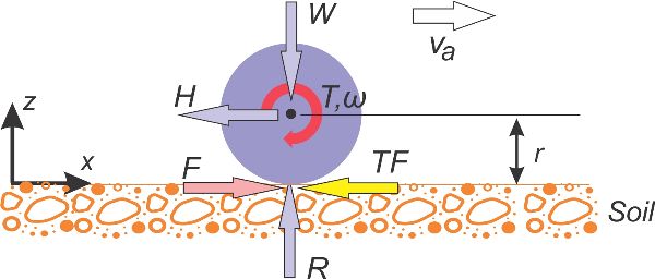
If the wheel represented in Figure 3.1.3 has no motion in the vertical direction (z axis), the wheel is in static equilibrium in this direction. In this condition, the summation of forces in the z (vertical) direction is zero. Therefore,
\[ \sum F_{z} = 0 \]
\[ R-W=0 \]
\[ R=W \]
where Fz = any force applied to the wheel in z direction (N)
R = vertical reaction force of the wheel (N)
If the actual speed of the wheel represented in Figure 3.1.3 is constant, the horizontal forces are in static equilibrium in this direction and the sum of the horizontal forces is zero. Therefore,
\[ \sum F_{x}=0 \]
where Fx = any force applied to the wheel in x direction (N)
F = gross tractive force (N)
Fr = motion resistance force (N)
Based on Equation 3.1.12, the gross tractive force (F) must be the net tractive force (H) plus the motion resistance force (Fr). If both sides of Equation 3.1.12 are divided by the dynamic load (W) acting on the wheel, resulting in Equation 3.1.13, three dimensionless numbers, i.e., μn, μg, and ρ, are created as shown in Equations 3.1.15, 3.1.16, and 3.1.17. The first one is the net traction ratio (μn), defined as the net tractive force divided by the dynamic load. The second one is the gross traction ratio (μg), defined as the gross tractive force divided by the dynamic load. And the third one is the motion resistance ratio (μ), defined as the motion resistance force divided by the dynamic load.
\[ \frac{H}{W}=\frac{F}{W}-\frac{F_{r}}{W} \]
Equation 3.1.14 shows that μn, μg, and ρ are not independent. By using a technique called dimensional analysis, functions were developed to predict how μg and ρ change as a function of the wheel variables and soil resistance. This analysis is presented by Goering et al. (2003) and is beyond the scope of this chapter. If μg, ρ, and W are known, the tractive force generated by the wheel can be predicted using Equation 3.1.18:
\[ H= (\mu_{g}-\rho)W \]
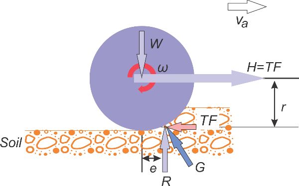
The R, F, and Fr forces (Figure 3.1.3) act on a point called the wheel resistance center. This point is not aligned with the direction of the dynamic load W but is a little bit ahead of it. This horizontal distance is called the horizontal offset (e). The static analysis of a towed wheel (Figure 3.1.4) shows that the wheel resistance center is not aligned with the direction of the dynamic wheel load. In a towed wheel, there is no torque applied to its axle. The soil reaction (G) at the resistance center is the resultant of the R and Fr forces. The direction of the G force passes through the wheel center. To move the towed wheel at a constant actual velocity (va), a net tractive force (H) equal to the motion resistance force (Fr) needs to be applied to the wheel. For the wheel to keep an angular velocity constant, the sum of the momentums at the center of the wheels must equal zero. Goering et al. (2003) showed that the horizontal offset can be calculated with Equations 3.1.19-3.1.21.
\[ Re-F_{r}r = 0 \]
where e = horizontal offset (m).
By using Equation 3.1.18, the tractive force can be predicted. The other important information in the wheel traction analysis is to predict how much torque needs to be transferred to the wheel axle to generate the tractive force (H). In Equation 3.1.5, the wheel radius is used to convert the rotational angular velocity to the theoretical wheel velocity. The wheel radius can also be used to calculate the torque necessary to produce the wheel tractive force. The torque (T) necessary to keep the angular velocity of the wheel constant and produce the net tractive force is the product of the gross tractive force and the torque radius of the wheel, as given by:
where rt = torque radius of the wheel (m).
The wheel radius defined in Equation 3.1.5 is different from the torque radius of the wheel defined in Equation 3.1.22 because of the interaction of the wheel and the surface, which varies on a soft soil surface. Generally, a rolling radius based on the distance from the center of the wheel axle to a hard surface is used. Therefore, Equation 3.1.23 can be used to estimate the torque acting at wheel axle:
\[ T=Fr \]
Engine Power Needed to Produce a Tractive Force
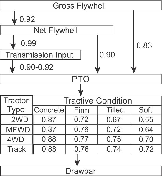
ASABE Standards (2015) presented a diagram (Figure 3.1.5) of the approximate typical power relationship for agricultural tractors. Tractors can be specified by their engine gross flywheel rated power (Pe). One of the standards used to define the engine gross flywheel rated power is SAE J1995 (SAE, 1995). The rated power defined by this standard is the mechanical power produced by the engine without some of its accessories (such as the alternator, the radiator fan, and the water pump). Therefore, the engine gross flywheel rated power is greater than the net power produced by the engine. The approximate engine net flywheel power can be estimated by multiplying the gross flywheel power by 0.92. The power at the tractor PTO is about equal to the engine gross flywheel power multiplied by 0.83 or the engine net flywheel power multiplied by 0.90.
The power that the tractor can generate to pull implements, often termed drawbar power because many implements are attached to the tractor’s drawbar, depends on the tractor type, i.e., 2-wheel drive (2WD), mechanical front wheel drive (MFWD), 4-wheel drive (4WD), or tracked. The surface condition where the tractor is used has an even greater effect. Using these two pieces of information, coefficients that show estimates of the relationship between the drawbar power and the PTO power is given in Figure 3.1.5.
The drawbar power required to pull an implement is:
\[ P_{DB} = F_{i} \nu_{i} \]
where PDB = drawbar power (W)
Fi = force required to pull an implement (N)
vi = implement velocity (m s−1)
The force required to pull an implement depends on the implement. For example, the force required to pull a planter Fp is the force required per row times the number of rows:
\[ F_{p} = f_{r}n_{r} \]
where fr = force required per row of planter (N row−1)
nr = number of rows
Once the required drawbar power is determined, the values in Figure 3.1.5 can be used to calculate the estimated needed gross flywheel rated power of a tractor to pull the implement.
Applications
The concepts of traction and tractor power are necessary for properly matching the tractor to an implement. Agricultural operations cannot be performed if the tractor cannot develop enough power or traction to pull the implement. As implements have increased in size over the years, it is necessary that the tractors have enough power and enough traction for the tasks they have to perform. Choosing a tractor that is too large will negatively impact agricultural profitability because larger tractors cost more than smaller tractors. An oversize tractor may also increase fuel consumption and exhaust emissions. This is significant because even the most efficient tractors get less than 4 kWh of work per liter of diesel fuel.
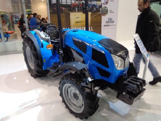
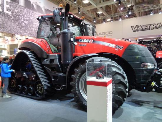
Tractors range greatly in size (e.g., Figure 3.1.6). For example, one large contemporary manufacturer sells tractors from 17 to 477 kW. The weight of the tractor must be enough to generate sufficient traction force, as shown in Equation 3.1.18. However, besides the cost of adding weight, additional weight may increase soil compaction and depress crop yields. It is therefore necessary to understand these concepts to design tractors and implements. The capabilities of the tractor’s engine, power transmission elements, and wheels need to be appropriately scaled. There needs to be a trade-off between making them large and powerful with making them compact and inexpensive. The above analyses can be used to guide tractor choice and design.
The concepts are also applied to other types of agricultural machinery, such as self-propelled harvesters and sprayers. For these machines to be able to complete their tasks, they need to be able to move across agricultural soils. The same calculations can be used to determine if there is enough power and to design the various components on those machines. The wheels, axles, and power transmission components must be able to withstand the forces, torques, and power during the machines’ use.
Examples
Example \(\PageIndex{1}\)
Example 1: Tractive force
Problem:
Calculate the tractive force produced by a tractor wheel that works on a firm soil with a dynamic load of 5 kN. The wheel velocity is 2 m s−1. If the tractive efficiency is 0.73, what is the power that needs to be transferred to the wheel axle?
Solution
Assume an equivalent coefficient of friction of 0.48, the mean value for firm soil presented in Table 3.1.1. Calculate the tractive force using Equation 3.1.4:
\( H= \mu W=0.48 \times 5 = 2.4 \text{ kN} \)
Now, calculate the tractive power for the tractor wheel using Equation 3.1.2:
\( P_{t} = H\nu_{a} = 2.4 \times 2 = 4.8 \text{ kW} \)
Calculate the power that needs to be transferred to the wheel axle for using Equation 3.1.3 with the given tractive efficiency of 0.73:
\( P_{W} = \frac{P_{t}}{T_{E}} = \frac{4.8}{0.73} = 6.58 \text{ kW} \)
This value of needed power can be used to design the various power transmission components. The power consumption can also be used to calculate the power demanded of the ultimate power source, probably an engine, to calculate fuel consumption and, thereby, costs of a particular field operation.
Example \(\PageIndex{2}\)
Example 2: Torque and travel reduction ratio, or slip
Problem:
A wheel on another tractor receives 40 kW from the tractor powertrain. The wheel rotates at 25 rpm, which is an angular velocity, ω, of 2.62 rad s−1. (Note: 2π rad × 25 rpm/60 min s−1 = 2.62 rad s−1.) If the rolling radius of the wheels is 0.81 m and the speed of the tractor is 2 m s−1, calculate the torque acting on the wheel and the travel reduction ratio (commonly known as slip).
Solution
Calculate the torque acting on the wheel T for a power Pw of 40 kW using Equation 3.1.1:
\( T=\frac{P_{W}}{\omega} = \frac{40}{2.62} = 15.28 \text{ Nm} \)
Calculate the power to be transferred to the wheel for producing 2.4 kN of tractive force at 2 m s−1 of wheel speed using Equation 3.1.3:
\( P_{W} = \frac{P_{t}}{T_{E}} = \frac{4.8}{0.73} =6.58 \text{ kW} \)
Calculate the theoretical velocity of the wheel vt for a rolling radius r of 0.81 m using Equation 3.1.5:
\( \nu_{t} = \omega r = 2.62 \times 0.81 = 2.12 \text{ m}s^{-1} \)
Since the actual velocity of the wheel is 2 m s−1, which is less than the theoretical velocity of the wheel, calculate the travel reduction ratio s using Equation 3.1.6:
\( s= \frac{\nu_{t}-\nu_{a}}{\nu_{t}} = \frac{2.12-2.00}{2.12} = 0.057, \text{or} \ 5.7\% \)
In addition to providing guidance to the design of the agricultural machine and its power consumption, calculation of the slip is useful to determine how fast the operation will be performed. Excessive slip can also have adverse effects on the soil’s structure and inhibit plant growth.
Example \(\PageIndex{3}\)
Example 3: Tractive force and power
Problem:
Consider a wheel that works with a dynamic load of 10 kN, a motion resistance ratio of 0.08, and a gross traction ratio of 0.72. Find the tractive force that the wheel can develop. If this wheel rotates at 40 rpm and the rolling radius of the wheel is 0.71 m, how much power is necessary to move this wheel?
Solution
Calculate the gross tractive force developed by the wheel F using Equation 3.1.16:
\( F= \mu_{g} W = 0.72 \times 10 = 7.2 \text{ kN} \)
Calculate the motion resistance Fr of this wheel using Equation 3.1.17:
\( F_{r} = \rho W = 0.08 \times 10 = 0.80 \text{ kN} \)
The tractive force H developed by the wheel, according to Equation 3.1.12, is the difference between the gross tractive force and the motion resistance:
\( H = F-F_{r} = 7.2 - 0.8 = 6.4 \text{ kN} \)
Calculate the torque necessary to move this wheel using Equation 3.1.23:
\( T = Fr = 7.2 \times 0.71 = 5.11 \text{ kN m} \)
Calculate the power Pw necessary to turn the wheel using Equation 3.1.1:
\( P_{W} = T \omega = T \frac{2\pi N}{60} = 5.11 \times \frac{2 \times \pi \times 40}{60} = 21.4 \text{ kW} \)
Example \(\PageIndex{4}\)
Example 4: Engine gross flywheel power
Problem:
Calculate the necessary power of a MFWD tractor to pull a 30-row planter. According to ASABE Standards (2015), a force of 900 N per row is required to pull a drawn row crop planter if it is only performing the seeding operation. The speed of the tractor will be 8.1 km h−1 (2.25 m s−1). The soil is in the tilled condition. Consider that the tractor should have a power reserve of 20% to overcome unexpected overloads.
Solution
Calculate the drawbar force needed to pull the planter using Equation 3.1.25:
\( F_{p} = f_{r}n_{r} = 900 \times 30 = 27,000 \text{ N} \)
Calculate the drawbar power PDB needed to pull the planter using Equation 3.1.24:
\( P_{DB} = F_{p} \nu_{p} = 27,000 \times 2.25 = 60,750 \text{ W} \)
Therefore, the tractor needs to produce a drawbar power of 60.75 kW. From Figure 3.1.5, find that the coefficient that relates the drawbar power to the PTO power of the tractor for a MFWD tractor working on tilled soil condition is 0.72. Thus, the tractor PTO power PPTO should be:
\( P_{PTO} = \frac{P_{DB}}{0.72} = \frac{60.75}{0.72} = 84 \text{ kW} \)
Considering that the coefficient that relates the PTO power to the engine gross flywheel power is 0.83 (Figure 3.1.5), the engine gross flywheel power Pe is:
\( P_{e} = \frac{P_{PTO}}{0.83} = \frac{84.375}{0.83} = 102 \text{ kW} \)
Considering a reserve of power of 20% to overcome unexpected overloads, the tractor selected should have an engine gross flywheel power at least 20% greater than that needed to pull the 30-row planter, or 1.2 × 10² kW = 122 kW.
These calculations will help the farm manager select the proper tractor for the operation.
Image Credits
Figure 1. Queiroz, D. (CC By 4.0). (2020). Schematic view of a two-wheel drive agricultural tractor.
Figure 2. Queiroz, D. (CC By 4.0). (2020). Simplified diagram of the variables related to a wheel developing a net tractive force.
Figure 3. Queiroz, D. (CC By 4.0). (2020). Diagram of the variables related to a wheel developing a net tractive force (H) including the gross tractive force (F) and the motion resistance force (Fr).
Figure 4. Queiroz, D. (CC By 4.0). (2020). Diagram of forces acting on a towed wheel.
Figure 5. ASABE Standard ASAE D497.7 (CC By 4.0). (2020). Diagram of the approximate power relationships in agricultural tractors (types are defined in the main text) and soil conditions.
Figure 6. Schueller, J. (CC By 4.0). (2020). Typical contemporary (a) small and (b) large tractors.
References
ASABE Standards. (2018). ANSI/ASAE S296.5 DEC2003 (R2018): General terminology for traction of agricultural traction and transport devices and vehicles. St. Joseph, MI: ASABE.
ASABE Standards. (2015). ASAE D497.7 MAR2011 (R2015): Agricultural machinery management data. St. Joseph, MI: ASABE.
Goering, C. E., Stone, M. L., Smith, D. W., & Turnquist, P. K. (2003). Traction and transport devices. In Off-road vehicle engineering principles (pp. 351-382). St. Joseph, MI: ASAE.
Kolator, B., & Białobrzewski, I. (2011). A simulation model of 2WD tractor performance. Comput. Electron. Agric. 76(2): 231-239.
Renius, K. T. (2020). Fundamentals of tractor design. Cham, Switzerland: Springer Nature.
SAE. (1995). SAE J1995_199506: Engine power test code—Spark ignition and compression ignition—Gross power rating. Troy, MI: SAE.
Schueller, J. K. (2000). In the service of abundance: Agricultural mechanization provided the nourishment for the 20th century’s extraordinary growth. Mech. Eng. 122(8):58-65.