
3.4: Mechatronics and Intelligent Systems in Agricultural Machinery
- Page ID
- 46848

Francisco Rovira-Más
Agricultural Robotics Laboratory, Universitat Politècnica de València, Valencia, Spain
Qin Zhang
Center for Precision & Automated Agricultural Systems, Washington State University, Prosser, Washington
Verónica Saiz-Rubio
Agricultural Robotics Laboratory, Universitat Politècnica de València, Valencia, Spain
| Key Terms |
| Control systems | Analog and digital data | Auto-guided tractors |
| Actuators | Positioning | Variable-rate application |
| Sensors | Vision and imaging | Intelligent machinery |
Variables
Introduction
Visitors to local farm fairs have a good chance of seeing old tractors. Curious visitors will notice that the oldest ones, say, those made in the first three decades of the 20th century, are purely mechanical. As visitors observe newer tractors, they may find that electronic and fluid powered components appeared in those machines. Now, agricultural machinery, such as tractors and combines, are so sophisticated that they are fully equipped with electronic controls and even fancy flat screens. These controls and screens are the driver interface to electromechanical components integrated into modern tractors.
The term mechatronics is used to refer to systems that combine computer controls, electrical components, and mechanical parts. A mechatronics solution is not just the addition of sensors and electronics to an already existing machine; rather, it is the balanced integration of all of them in such a way that each individual component enhances the performance of the others. This outcome is achieved only by considering all subsystems simultaneously at the earliest stages of design (Bolton, 1999). Thus, mechatronics unifies the technologies that underlie sensors, automatic control systems, computing processors, and the transmission of power through mechanisms including fluid power actuators.
During the 20th century, agricultural mechanization greatly reduced the drudgery of farm work while increasing productivity (more land farmed by fewer people), efficiency (less time and resources invested to farm the same amount of land), and work quality (reduced losses at harvesting, more precise chemical applications, achieving uniform tillage). The Green Revolution, led by Norman Borlaug, increased productivity by introducing region-adapted crop varieties and the use of effective fertilizers, which often resulted in yields doubling, especially in developing countries. With such improvements initiated by the Green Revolution, current productivity, efficiency, and quality food crops may be sufficient to support a growing world population projected to surpass 9.5 billion by 2050, but the actual challenge is to do it in a sustainable way by means of a regenerative agriculture (Myklevy et al., 2016). This challenge is further complicated by the continuing decline of the farm workforce globally.
Current agricultural machinery, such as large tractors, sprayers, and combine harvesters, can be too big in practice because they must travel rural roads, use powerful diesel engines that are subjected to restrictive emissions regulations, are difficult to automate for liability reasons, and degrade farm soil by high wheel compaction. These challenges, and many others, may be overcome through the adoption of mechatronic technologies and intelligent systems on modern agricultural machinery. Mechanized farming has been adopting increased levels of automation and intelligence to improve management and increase productivity in field operations. For example, farmers today can use auto-steered agricultural vehicles for many different field operations including tilling, planting, chemical applications, and harvesting. Intelligent machinery for automated thinning or precise weeding in vegetable and other crops has recently been introduced to farmers.
This chapter introduces the basic concepts of mechatronics and intelligent systems used in modern agricultural machinery, including farming robots. In particular, it briefly introduces a number of core technologies, key components, and typical challenges found in agricultural scenarios. The material presented in this chapter provides a basic introduction to mechatronics and intelligent technologies available today for field production applications, and a sense of the vast potential that these approaches have for improving worldwide mechanization of agriculture in the next decades.
Concepts
The term mechatronics applies to engineering systems that combine computers, electronic components, and mechanical parts. The concept of mechatronics is the seamless integration of these three subsystems; its embodiment in a unique system leads to a mechatronic system. When the mechatronic system is endowed with techniques of artificial intelligence, the mechatronic system is further classified as an intelligent system, which is the basis of robots and intelligent farm machinery.
Automatic Control Systems
Machinery based on mechatronics needs to have control systems to implement the automated functions that accomplish the designated tasks. Mechatronic systems consist of electromechanical hardware and control software encoding the algorithm or model that automate an operation. An automatic control system obtains relevant information from the surrounding environment to manage (or regulate) the behavior of a device performing desired operations. A good example is a home air conditioner (AC) controller that uses a thermostat to determine the deviation of room temperature from a preset value and turn the AC on and off to maintain the home at the preset temperature. An example in agricultural machinery is auto-steering. Assume a small utility tractor has been modified to steer automatically between grapevine rows in a vineyard. It may use a camera looking ahead to detect the position of vine rows, such that deviations of the tractor from the centerline between vine rows are related to the proper steering angle for guiding the tractor in the vineyard without hitting a grapevine. From those two examples, it can be seen that a control system, in general, consists of sensors to obtain information, a controller to make decisions, and an actuator to perform the actions that automate an operation.
Actuation that relies on the continuous tracking of the variable under control (such as temperature or wheel angle) is called closed-loop control and provides a stable performance for automation. Closed-loop control allows the real-time estimation of the error (which is defined as the difference between the desired output of the controlled variable and the actual value measured by a feedback sensor), and calculates a correction command with a control function—the controller—for reducing the error. This command is sent to the actuator (discussed in the next section) for automatically implementing the correction. This controller function can be a simple proportion of the error (proportional controller, P), a measure of the sensitivity of change (derivative controller, D), a function dependent on accumulated (past) errors (integral controller, I), or a combination of two or three of the functions mentioned above (PD, PI, PID). There are alternative techniques for implementing automated controls, such as intelligent systems that use artificial intelligence (AI) methods like neural networks, fuzzy logic, genetic algorithms, and machine learning to help make more human-like control decisions.
Actuators
An electromechanical component is an integrated part that receives an electrical signal to create a physical movement to drive a mechanical device performing a certain action. Examples of electromechanical components include electrical motors that convert input electrical current into the rotation of a shaft, and pulse-width modulation (PWM) valves, such as variable rate nozzles and proportional solenoid drivers, which receive an electrical signal to push the spool of a hydraulic control valve to adjust the valve opening that controls the amount of fluid passing through. Because hydraulic implement systems are widely used on agricultural machinery, it is common to see many more electrohydraulic components (such as proportional solenoid drivers and servo drivers) than electrical motors on farm machines. However, as robotic solutions become increasingly more available in agriculture, applications of electrical motors on modern agricultural machinery will probably increase, especially on intelligent and robotic versions. The use of mechatronic components lays the foundation for adopting automation technologies to agricultural machinery, including the conversion of traditional machines into robotic ones capable of performing field work autonomously.
Intelligent Agricultural Machinery and Agricultural Robots
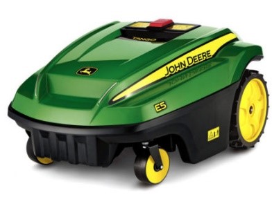
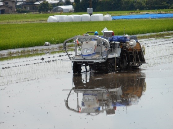
For intelligent agricultural machinery to be capable of performing automated field operations, it is required that machines have the abilities of: (1) becoming aware of actual operation conditions; (2) determining adaptive corrections suitable for continuously changing conditions; and (3) implementing such corrections during field operations, with the support of a proper mechanical system. The core for achieving such a capability often rests on the models that govern intelligent machinery, ranging from simple logic rules controlling basic tasks all the way to sophisticated AI algorithms for carrying out complex operations. These high-level algorithms may be developed using popular techniques such as artificial neural networks, fuzzy logic, probabilistic reasoning, and genetic algorithms (Russell and Norvig, 2003). As many of those intelligent machines could perform some field tasks autonomously, like a human worker could do, such machinery can also be referred to as robotic machinery. For example, when an autonomous lawn mower (Figure 3.4.1a) roams within a courtyard, it is typically endowed with basic navigation and path-planning skills that make the mower well fit into the category of robotic machinery, and therefore, it is reasonable to consider it a field robot. Though these robotic machines are not presently replacing human workers in field operations, the introduction of robotics in agriculture and their widespread use is only a matter of time. Figure 3.4.1b shows an autonomous rice transplanter (better called a rice transplanting robot) developed by the National Agriculture and Food Research Organization (NARO) of Japan.
(a)
(b)
Figure \(\PageIndex{1}\): (a) Autonomous mower (courtesy of John Deere); (b) GPS-based autonomous rice transplanter (courtesy of NARO, Japan).
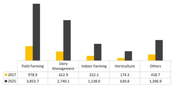
Many financial publications forecast that there will be a rapid growth of the market for service robots in the next two decades, and those within agricultural applications will play a significant role. Figure 3.4.2 shows the expected growth of the U.S. market for agricultural robots by product type. Although robots for milking and dairy management have dominated the agricultural robot market in the last decade, crop production robots are expected to increase their presence commercially and lead the market in the coming years, particularly for specialty crop production (e.g., tree fruit, grapes, melons, nuts, and vegetables). This transformation of the 21st century farmer from laborer to digital-age manager may be instrumental in attracting younger generations to careers in agricultural production.
Sensors in Mechatronic Systems
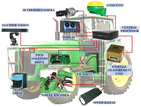
Sensors are a class of devices that measure significant parameters by using a variety of physical phenomena. They are important components in a mechatronic system because they provide the information needed for supporting automated operations. While the data to be measured can be in many forms, sensors output the measured data either in analog or digital formats (described in the next section). In modern agricultural machinery, sensor outputs are eventually transformed to digital format and thus can be displayed on an LCD screen or fed to a computer. This high connectivity between sensors and computers has accelerated the expansion of machinery automation. An intelligent machine can assist human workers in conducting more efficient operations: in some cases, it will simply entail retrieving clearer or better information; in other cases, it will include the automation of physical functions. In almost all situations, the contribution of reliable sensors is needed for machines to interact with the surrounding environment. Figure 3.4.3 shows the architecture of an intelligent tractor, which includes the typical sensors onboard intelligent agricultural machinery.
Even though sensors collect the data required to execute a particular action, that may not be enough because the environment of agricultural production is often complicated by many factors. For example, illumination changes throughout the day, adverse weather conditions may impair the performance of sensors, and open fields are rife with uncertainty where other machines, animals, tools, and even workers may appear unexpectedly in the near vicinity. Sensed data may be insufficient to support a safe, reliable, and efficient automated operation, and therefore data processing techniques are necessary to get more comprehensive information until it becomes sufficient to support automated operations. As a rule of thumb, there is no sensor that provides all needed information, and there is no sensor that never fails. Depending on specific needs, engineers often use either redundancy or sensor fusion to solve such a problem. The former acquires the same information through independent sources in case one of them fails or decreases in reliability, and the latter combines information of several sources that are complementary. Once the sensed information has been processed using either method, the actuation command can be calculated and then executed to complete the task.
Analog and Digital Data
As mentioned above, mechatronic systems often use sensors to obtain information to support automated operations. Sensors provide measurements of physical magnitudes (e.g., temperature, velocity, pressure, distance, and light intensity) represented by a quantity of electrical variables (such as voltages and currents). These quantities are often referred to as analog data and normally expressed in base 10, the decimal numbering system. In contrast, electronic devices such as controllers represent numbers in base 2 (the binary numbering system or simply “binary”) by adopting the on-off feature of electronics, with a numerical value of 1 assigned to the “on” state and 0 assigned to the “off” state.
A binary system uses a series of digits, limited to zeros or ones, to represent any decimal number. Each of these digits represents a bit of the binary number; a binary digit is called a bit. The leftmost 1 in the binary number 1001 is called the most significant bit (MSB), and the rightmost 1 is the least significant bit (LSB). It is common practice in computer science to break long binary numbers into segments of 8 bits, known as bytes. There is a one-to-one correspondence between binary numbers and decimal numbers. For instance, a 4-bit binary number can be used to represent all the positive decimal integers from 0 (represented by 0000) to 15 (represented by 1111). Signal digitization consists of finding that particular correspondence.
The process of transforming binary numbers to decimal numbers and vice versa is straightforward for representing positive decimal integers. However, negative and floating-point numbers require special techniques. While the transformation of data between two formats is normally done automatically, it is important to know the underlying concept for a better understanding of how information can be corrected, processed, distributed, and utilized in intelligent machinery systems. The resolution of digital data depends on the number of bits, such that more bits means more precision in the digitized measurement. Equation 3.4.1 yields the relationship between the number of bits (n) and the resulting number of digital levels available to code the signal (L). For example, using 4 bits leads to 24 = 16 levels, which implies that an analog signal between 0 V and 2 V will have a resolution of 2/15 = 0.133 V; as a result, quantities below 133 mV will not be detected using 4-bit numbers. If more accuracy is necessary, digitization will have to use numbers with more bits. Note that Equation 3.4.1 is an exponential relationship rather than linear, and quantization grows fast with the number of bits. Following with the previous example, 4 bits produce 16 levels, but 8 bits give 256 levels instead of 32, which actually corresponds to 5 bits.
\[ L=2^{n} \]
where L = number of digital levels in the quantization process
n = number of bits
Position Sensing
One basic requirement for agricultural robots and intelligent machinery to work properly, reliably, and effectively is to know their location in relation to the surrounding environment. Thus, positioning capabilities are essential.
Global Navigation Satellite Systems (GNSS)
Global Navigation Satellite System (GNSS) is a general term describing any satellite constellation that provides positioning, navigation, and timing (PNT) services on a global or regional basis. While the USA Global Positioning System (GPS) is the most prevalent GNSS, other nations are fielding, or have fielded, their own systems to provide complementary, independent PNT capability. Other systems include Galileo (Europe), GLONASS (Russia), BeiDou (China), IRNSS/NavIC (India), and QZSS (Japan).
When the U.S. Department of Defense released the GPS technology for civilian use in 2000, it triggered the growth of satellite-based navigation for off-road vehicles, including robotic agricultural machinery. At present, most leading manufacturers of agricultural machinery include navigation assistance systems among their advanced products. As of 2019, only GPS (USA) was fully operational, but the latest generation of receivers can already expand the GPS constellation with other GNSS satellites.
GPS receivers output data through a serial port by sending a number of bytes encoded in a standard format that has gained general acceptance: NMEA 0183. The NMEA 0183 interface standard was created by the U.S. National Marine Electronics Association (NMEA), and consists of GPS messages in text (ASCII) format that include information about time, position in geodetic coordinates (i.e., latitude (λ), longitude (φ), and altitude (h)), velocity, and signal precision. The World Geodetic System 1984 (WGS 84), developed by the U.S. Department of Defense, defines an ellipsoid of revolution that models the shape of the earth, and upon which the geodetic coordinates are defined. Additionally, the WGS 84 defines a Cartesian coordinate system fixed to the earth and with its origin at the center of mass of the earth. This system is the earth-centered earth-fixed (ECEF) coordinate system, and it provides an alternative way to locate a point on the earth surface with the conventional three Cartesian coordinates X, Y, and Z, where the Z-axis coincides with the earth’s rotational axis and therefore crosses the earth’s poles.
The majority of the applications developed for agricultural machinery, however, do not require covering large surfaces in a short period of time. Therefore, the curvature of the earth has a negligible effect, and most farm fields can be considered flat for practical purposes. A local tangent plane coordinate system (LTP), also known as NED coordinates, is often used to facilitate such small-scale operations with intuitive global coordinates north (N), east (E), and down (D). These coordinates are defined along three orthogonal axes in a Cartesian configuration generated by fitting a tangent plane to the surface of the earth at an arbitrary point selected by the user and set as the LTP origin. Given that standard receivers provide geodetic coordinates (λ, φ, h) but practical field operations require a local frame such as LTP, a fundamental operation for mapping applications in agriculture is the real-time transformation between the two coordinate systems (Rovira-Más et al., 2010). Equations 3.4.2 to 3.4.8 provide the step by step procedure for achieving this transformation.
\[ a = 6378137 \]
\[ e = 0.0818 \]
\[ N_{0}(\lambda)=\frac{a}{\sqrt{1-e^{2} \cdot sin^{2}\lambda}} \]
\[ X=(N_{0}+h) \cdot cos\lambda \cdot cos\phi \]
\[ Y=(N_{0}+h) \cdot cos\lambda \cdot sin\phi \]
\[ Z=[h+N_{0} \cdot (1-e^{2})] \cdot sin\lambda \]
\[ \begin{bmatrix} N \\E\\D \end{bmatrix} = \begin{bmatrix} -sin \lambda \cdot cos\phi & -sin\lambda \cdot sin\phi & cos\lambda \\ -sin\phi &cos\phi & 0 \\ -cos\lambda \cdot cos\phi & -cos\lambda \cdot sin\phi & -sin\lambda \end{bmatrix} \cdot \begin{bmatrix} X-X_{0} \\ Y-Y_{0} \\ Z-Z_{0} \end{bmatrix} \]
where a = semi-major axis of WGS 84 reference ellipsoid (m)
e = eccentricity of WGS 84 reference ellipsoid
N0 = length of the normal (m)
Geodetic coordinates:
λ= latitude (°)
φ = longitude (°)
h = altitude (m)
(X, Y, Z) = ECEF coordinates (m)
(X0, Y0, Z0) = user-defined origin of coordinates in ECEF format (m)
(N, E, D) = LTP coordinates north, east, down (m)
Despite the high accessibility of GPS information, satellite-based positioning is affected by a variety of errors, some of which cannot be totally eliminated. Fortunately, a number of important errors may be compensated by using a technique known as differential correction, lowering errors from more than 10 m to about 3 m. Furthermore, the special case of real-time-kinematic (RTK) differential corrections may further lower error to just centimeter level.
Sonar Sensors
In addition to locating machines in the field, another essential positioning need for agricultural robots is finding the position of surrounding objects during farming operations, such as target plants or potential obstacles. Ultrasonic rangefinders are sensing devices used successfully for this purpose. Because they measure the distance of target objects in terms of the speed of sound, these sensors are also known as sonar sensors.
The underlying principle of sonars is that the speed of sound is known (343 m s−1 at 20°C), and measuring the time that the wave needs to hit an obstacle and return to the sensor—the echo—allows the estimation of an object’s distance. The speed of sound through air, V, depends on the ambient temperature, T, as:
\[ V(m\ s^{-1})=331.3 + 0.606 \times T(^\circ C) \]
The continuously changing ambient temperature in agricultural fields is one of many challenges to sonar sensors. Another challenge is the diversity of target objects. In practice, sonar sensors must send out sound waves that hit an object and then return to the sensor receiver. This receiver must then capture the signal to measure the elapsed time for the waves to complete the round trip. Understanding the limitations posed by the reflective properties of target objects is essential to obtain reliable results. The distance to materials that absorb sound waves, such as stuffed toys, will be measured poorly, whereas solid and dense targets will allow the system to perform well. When the target object is uneven, such as crop canopies, the measurements may become noisy. Also, sound waves do not behave as linear beams, but propagate in irregular cones that expand in coverage with distance. When objects are outside the cone, they may be undetected. Errors will often vary with ranges such that farther ranges lead to larger errors.
An important design feature to consider is the distance between adjacent ultrasonic sensors, as echo interference is another source of unstable behavior. Overall, sonar rangefinders are helpful to estimate short distances cost-efficiently when accuracy and reliability are not critical, as when detecting distances to the canopy of trees for automated pesticide spraying.
Light Detection and Ranging (Lidar) Sensors
Another common position-detecting sensor is lidar, which stands for light detection and ranging. Lidars are optical devices that detect the distance to target objects with precision. Although different light sources can be used to estimate ranges, most lidar devices use laser pulses because their beam density and coherency result in high accuracy.
Lidars possess specific features that make them favorable for field robotic applications, as sunlight does not affect lidars unless it hits their emitter directly, and they work excellently under poor illumination.
Machine Vision and Imaging Sensors
One important element of human intelligence is vision, which gives farmers the capability of visual perception. A basic requirement for intelligent agricultural machinery (or agricultural robots) is to have surrounding awareness capability. Machine vision is the computer version of the farmer’s sight; the cameras function as eyes and the computers as the brain. The output data of vision systems are digital images. A digital image consists of little squares called pixels (picture elements) that carry information on their level of light intensity. Most of the digital cameras used on agricultural robots are CCD (charge coupled devices), which are composed of a small rectangular sensor made of a grid of tiny light-sensitive cells, each of them producing the information of its corresponding pixel in the image. If the image is in black and white (technically called monochrome), the intensity level is represented in a gray scale between a minimum value (0) and a maximum value (imax). The number of levels in the gray scale depends on the number of bits in which the image is coded. Most of the images used in agriculture are 8 bits, which means that the image can distinguish 256 gray levels (28), where the minimum value is 0 representing complete black, and the maximum value is 255 representing pure white. In practical terms, human eyes cannot distinguish so many levels, and 8 bits are many times more than enough. When digital images reproduce a scene in color, pixels carry information of intensity levels for the three channels of red (R), green (G), and blue (B), leading to RGB images. The processing of RGB images is more complicated than monochrome images and falls outside the scope of this chapter.
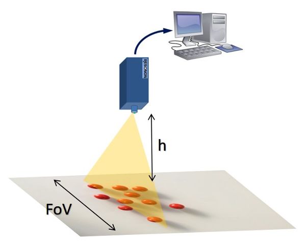
Monocular cameras (which have one lens) constitute simple vision systems, yet the information they retrieve is powerful. When selecting a camera, engineers must choose important technical parameters such as the focal length of the lens, the size of the sensor, and optical filters when there are spectral ranges (colors) that need to be blocked from the image. The focal length (f) is related to the scope of scene that fits into the image, and is defined in Equation 3.4.10. The geometrical relationship described by Figure 3.4.4 and Equation 3.4.11 determines the resulting field of view (FOV) of any given scene. The design of a machine vision system, therefore, must include the right camera and lens parameters to assure that the necessary FOV is covered and the target objects are in focus in the images.
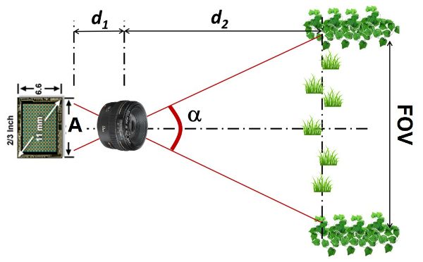
\[ \frac{1}{f} = \frac{1}{d_{1}}+\frac{1}{d_{2}} \]
\[ \frac{d_{1}}{d_{2}} = \frac{A}{FOV} \]
where f = lens focal length (mm)
d1 = distance between the imaging sensor and the optical center of the lens (mm)
d2 = distance between the optical center of the lens and the target object (mm)
A = horizontal dimension of the imaging sensor (mm)
FOV = horizontal field of view covered in the images (mm)
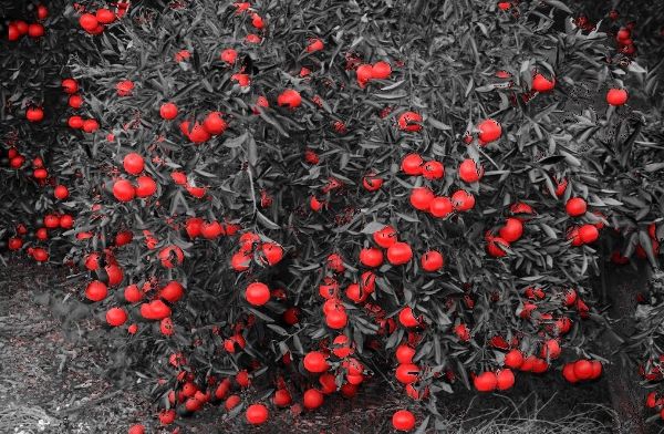
After taking the images, the first step of the process (image acquisition) is complete. The second step, analysis of the images, begins with image processing, which involves the delicate task of extracting the useful information from each image for its later use. Figure 3.3.5 reproduces the results of a color-based segmentation algorithm to find the position of mandarin oranges in a citrus tree.
Even though digital images reproduce scenes with great detail, the representation is flat, that is, in two dimensions (2D). However, real scenes are in three dimensions (3D), with the third dimension being the depth, or distance between the camera and the objects of interest in the scene. In the image shown in Figure 3.3.5, for instance, a specific orange can be located with precision in the horizontal and vertical axes, but how far it is from the sensor cannot be known. This information would be essential, for example, to program a robotic arm to retrieve the oranges. Stereo cameras (which are cameras with at least two lenses that meet the principles of stereoscopy) allow the acquisition of two (or more) images in a certain relative position to which the principles of stereoscopic vision apply. These principles mimic how human vision works, as the images captured by human eyes in the retinas are slightly offset, and this offset (known as disparity) is what allows the brain to estimate depth.
Estimation of Vehicle Dynamic States
The parameters that help understand a vehicle’s dynamic behavior are known as the vehicle states, and typically include velocity, acceleration, sideslip, and angular rates yaw, pitch, and roll. The sensors needed for such measurements are commonly assembled in a compact motion sensor called an inertial measurement unit (IMU), created from a combination of accelerometers and gyroscopes. The accelerometers of the IMU detect acceleration as the change in velocity of the vehicle over time. Once the acceleration is known, its mathematical integration gives an estimate of the velocity, and integrating again gives an estimate of the position. Equation 3.4.12 allows the calculation of instantaneous velocities from the acceleration measurements of an IMU or any individual accelerometer. Notice that for finite increments of time ∆t, the integral function is replaced by a summation. Similarly, gyroscopes can detect the angular rates of the turning vehicle; integrating these values leads to roll, pitch, and yaw angles, as specified by Equation 3.4.13. A typical IMU is composed of three accelerometers and three gyroscopes assembled along three perpendicular axes that reproduce a Cartesian coordinate system. With this physical configuration, it is possible to calculate the three components of acceleration and speed in Cartesian coordinates as well as Euler angles roll, pitch, and yaw. Current IMUs on the market are small and inexpensive, favoring the accurate estimation of vehicle states with small devices such as microelectromechanical systems (MEMS).
where Vt = velocity of a vehicle at time t (m s−1)
at = linear acceleration recorded by an accelerometer (or IMU) at time t (m s−2)
∆t = time interval between two consecutive measurements (s)
\(\Theta_{t}\) = angle at time t (rad)
\(\dot{\Theta}\) = angular rate at time t measured by a gyroscope (rad s−1)
Applications
Mechatronic Systems in Auto-Guided Tractors
As mentioned early in this chapter, mechatronic systems are now playing an essential role in modern agricultural machinery, especially on intelligent and robotic vehicles. For example, the first auto-guided tractors hit the market at the turn of the 21st century; from a navigation standpoint, farm equipment manufacturers have been about two decades ahead of the automotive industry. Such auto-guided tractors would not be possible if they had not been upgraded to state-of-the-art mechatronic systems, which include sensing, controlling, and electromechanical (or electrohydraulic) actuating elements. One of the most representative components never seen before on conventional mechanical tractors as an integrated element is the high-precision GPS receiver, which furnishes tractors with the capability to locate themselves in order to guide them following designated paths.
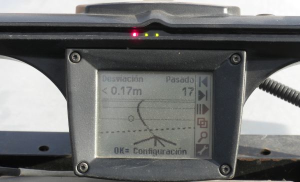
Early navigation solutions that were commercially available did not actually control the tractor steering system; rather, they provided tractor drivers with lateral corrections in real time, such that by following these corrections the vehicle easily tracked a predefined trajectory. This approach is easy to learn and execute, as drivers only need to follow a light-bar indicator, where the number of lights turned on is proportional to the sidewise correction to keep the vehicle on track. In addition to its simplicity of use, this system works for any agricultural machine, including older ones. Figure 3.4.6a shows a light-bar system mounted on an orchard tractor, where the red light signals the user to make an immediate correction to remain within the trajectory shown on the LCD screen.
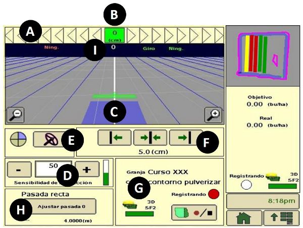
Another essential improvement of modern tractors based on mechatronics technology is the electrohydraulic system that allows tractors to be maneuvered by wire. This means that an operation of the tractor, such as steering or lowering the implement installed on the three-point hitch, can be accomplished by an electronically controlled electrohydraulic actuating system in response to control signals generated by a computer-based controller. An electrohydraulic steering system allows a tractor to be guided automatically, by executing navigation commands calculated by an onboard computer based on received GPS positioning signals. One popular auto-steering application is known as parallel tracking, which allows a tractor being driven automatically to follow desired pathways in parallel to a reference line between two points, say A-B line, in a field recorded by the onboard GPS system. These reference lines can even include curved sectors. Figure 3.4.6b displays the control screen of a commercial auto-guidance system implemented in a wheel-type tractor. Notice the magnitude of the tractor deviation (the off-track error) from the predefined trajectory is shown at the top bar, in a similar fashion as the corrections conveyed through light-bars. The implementation of automatic guidance has reduced pass-to-pass overlaps, especially with large equipment, resulting in significant savings in seeds, fertilizer, and phytosanitary chemicals as well as reduced operator fatigue. Farmers are seeing returns on investment in just a few years.
(a)
(b)
Figure \(\PageIndex{6}\): Auto-guidance systems: (a) Light-bar kit; (b) Parallel tracking control screen, where A is the path accuracy indicator, B is the off-track error, C represents the guidance icon, D provides the steering sensitivity, E mandates steer on/off, F locates the shift track buttons, G is the GPS status indicator, H is the A-B (0) track button, and I shows the track number.
Automatic Control of Variable-Rate Applications
The idea of variable rate application (VRA) is to apply the right amount of input, i.e., seeds, fertilizers, and pesticides, at the right time and at sub-plot precision, moving away from average rates per plot that result in economic losses and environmental threats. Mechatronics enables the practical implementation of VRA for precision agriculture (PA). Generally speaking, state-of-the-art VRA equipment requires three key mechatronic components: (1) sensors, (2) controllers, and (3) actuators.
Sub-plot precision is feasible with GPS receivers that provide the instantaneous position of farm equipment at a specific location within a field. In addition, vehicles require the support of an automated application controller to deliver the exact amount of product. The specific quantity of product to be applied at each location is commonly provided by either a prescription map preloaded to the vehicle’s computer, or alternatively, estimated in real time using onboard crop health sensors.
There are specific sensors that must be part of VRA machines. For example, for intelligent sprayers to be capable of automatically adapting the rate of pesticide to the properties of trees, global and local positioning in the field or related to crops is required. Fertilizers, on the other hand, may benefit from maps of soil parameters (moisture, organic matter, nutrients), as well as vegetation (vigor, stress, weeds, temperature). In many modern sprayers, pressure and flow of applied resources (either liquid or gaseous) must be tracked to support automatic control and eventually achieve a precise application rate. Controllers are the devices that calculate the optimal application rate on the fly and provide intelligence to the mechatronics system. They often consist of microcontrollers reading sensor measurements or loaded maps to calculate the instantaneous rate of product application based on internal algorithms. This rate is continuously sent to actuators for the physical application of product. Controllers may include small monitoring displays or switches for manual actuation from the operator cabin, if needed. Actuators are electromechanical or electrohydraulic devices that receive electrical signals from the controllers to regulate the amount of product to apply. This regulation is usually achieved by varying the rotational speed of a pump, modifying the flow coming from a tank, or changing the settings of a valve to adjust the pressure or flow of the product. Changing the pressure of sprayed liquids, however, results in a change of the droplet size, which is not desirable for pest control. In these cases, the use of smart nozzles that are controlled through PWM signals is recommended.
As VRA technology is progressing quickly, intelligent applicators are becoming available commercially, mainly for commodity crops. An intelligent system can automatically adjust the amount of inputs dispersed in response to needs, even permitting the simultaneous use of several kinds of treatments, resulting in new ways of managing agricultural production. For example, an intelligent VRA seeder has the ability to change the number of seeds planted in the soil according to soil potential, either provided by prescription maps or detected using onboard sensors. Control of the seeding rate is achieved by actuating the opening of the distributing device to allow the desired number of seeds to go through.
In many cases, a feedback control system is required to achieve accurate control of the application rate. For example, in applying liquid chemicals, the application rate may be affected by changes in the moving speed of the vehicle, as well as the environmental conditions. Some smart sprayers are programmed to accurately control the amount of liquid chemical by adjusting the nozzles in response to changes of sprayer forward speed. This is normally accomplished using electronically controlled nozzle valves that are commanded from the onboard processor. Such a mechatronic system could additionally monitor the system pressure and flow in the distribution circuit with a GPS receiver, and even compensate changes of the amount of liquid exiting the nozzles resulting from pressure or flow pattern changes in the circuit.
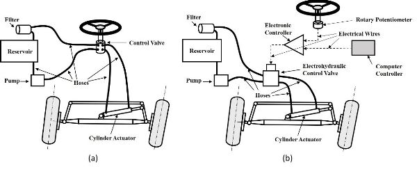
Redesigning a Tractor Steering System with Electrohydraulic Components
Implementing auto-guidance capabilities in a tractor requires that the steering system can be controlled electrically for automated turning of the front wheels. Therefore, it is necessary to replace a traditional hydraulic steering system with an electrohydraulic system. This could be accomplished simply by replacing a conventional manually actuated steering control valve (Figure 3.4.7a) by an electrohydraulic control system. Such a system (Figure 3.4.7b) consists of a rotary potentiometer to track the motion of the steering wheel, an electronic controller to convert the steering signal to a control signal, and a solenoid-driven electrohydraulic control valve to implement the delivered control signal.
The upgraded electrohydraulic steering system can receive control signals from a computer controller enabled to create appropriate steering commands in terms of outputs from an auto-guided system, making navigation possible without the input of human drivers to achieve autonomous operations with the tractor. As the major components of an electrohydraulic system are connected by wires, such an operation is also called “actuation by wire.”
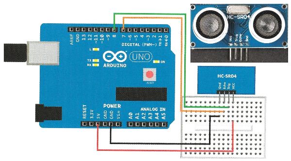
Use of Ultrasonic Sensors for Measuring Ranges
Agricultural machinery often needs to be “aware” of the position of objects in the vicinity of farming operations, as well as the position of the machinery. Ultrasonic sensors are often used to perform such measurements.
In order to use an ultrasonic (or sonar) sensor, a microprocessor is often needed to convert the analog signals (which are in the range of 0–5 V) from the ultrasonic sensor to digital signals, so that the recorded data can be further used by other components of automated or robotic machinery. For an example consider the HC-SR04, which consists of a sound emitter and an echo receiver such that it measures the time elapsed between a sound wave being sent by the emitter and its return back from the targeted object. The speed of sound is approximately 330 m·s−1, which means that it needs 3 s for sound to travel 1,000 m. The HC-SR04 sensor can measure ranges up to 4.0 m, hence the time measurements are in the order of milliseconds and microseconds for very short ranges. The sound must travel through the air, and the speed of sound depends on environmental conditions, mainly the ambient temperature. If this sensor is used on a hot summer day with an average temperature of 35°C, for example, using Equation 3.4.9, the corrected sound speed will be slightly higher, at 352 m·s−1.
Figure 3.4.8 shows how the sensor was connected to and powered by a commercial product (Arduino Uno microprocessor, for illustration purposes) in a laboratory setup (also for illustration). After completing all the wiring of the system as shown in Figure 3.4.8, it is necessary to select an unused USB port and any of the default baud rates in the interfacing computer. If the baud rate and serial port are properly set in a computer with a display console, and the measured ranges have been set via software at an updating frequency of 1 Hz, the system could then perform one measurement per second. After the system has been set up, it is important to check its accuracy and robustness by moving the target object in the space ahead of the sensor.
Examples
Example \(\PageIndex{1}\)
Example 1: Digitization of analog signals
Problem:
Mechatronic systems require sensors to monitor the performance of automated operations. Analog sensors are commonly used for such tasks. A mechatronics-based steering mechanism uses a linear potentiometer to estimate the steering angle of an auto-guided tractor, outputting an analog signal in volts as the front wheels rotate. To make the acquired data usable by a computerized system to automate steering, it is necessary to convert the analog data to digital format.
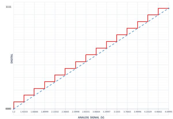
Given the analog signal coming from a steering potentiometer, digitize the signal using 4 bits of resolution, by these steps.
- 1. Calculate the number of levels coded by the 4-bit signal taking into account that the minimum voltage output by the potentiometer is 1.2 V and the maximum voltage is limited to 4.7 V, i.e., any reading coming from the potentiometer will belong to the interval 1.2 V–4.7 V. How many steps comprise this digital signal?
- 2. Establish a correspondence between the analog readings within the interval and each digital level from 0000 to 1111, drafting a table to reflect the correlation between signals.
- 3. Plot both signals overlaid to graphically depict the effect of digitizing a signal and the loss of accuracy behind the process. According to the plot, what would be the digital value corresponding to a potentiometer reading of 4.1 V?
Solution
The linear potentiometer has a rod whose position varies from retraction (1.2 V) to full extension (4.7 V). Any rod position between both extremes will correspond to a voltage in the range 1.2 V–4.7 V. The number of levels L encoded in the signal for n = 4 bits is calculated using Equation 3.4.1:
\( L=2^{n}=2^{4} = \textbf{16 levels} \)
Thus, the number of steps between the lowest digital number 0000 and the highest 1111 is 15 intervals. Table 3.4.1 specifies each digital value coded by the 4-bit signal, taking into account that the size of each interval ∆V is set by:
| Bit | 4-Bit Digital Signal | Analog Equivalence (V) | |||
|---|---|---|---|---|---|
| 1 | 2 | 3 | 4 | ||
|
1 |
1 |
1 |
1 |
1 1 1 1 |
4.70000 |
|
0 |
1 1 1 0 |
4.46666 |
|||
|
0 |
1 |
1 1 0 1 |
4.23333 |
||
|
0 |
1 1 0 0 |
4.00000 |
|||
|
0 |
1 |
1 |
1 0 1 1 |
3.76666 |
|
|
0 |
1 0 1 0 |
3.53333 |
|||
|
0 |
1 |
1 0 0 1 |
3.30000 |
||
|
0 |
1 0 0 0 |
3.06666 |
|||
|
0 |
1 |
1 |
1 |
0 1 1 1 |
2.83333 |
|
0 |
0 1 1 0 |
2.60000 |
|||
|
0 |
1 |
0 1 0 1 |
2.36666 |
||
|
0 |
0 1 0 0 |
2.13333 |
|||
|
0 |
1 |
1 |
0 0 1 1 |
1.90000 |
|
|
0 |
0 0 1 0 |
1.66666 |
|||
|
0 |
1 |
0 0 0 1 |
1.43333 |
||
|
0 |
0 0 0 0 |
1.20000 |
|||
\( \Delta V = (4.7 - 1.2)/15 = 3.5/15 = 0.233 V \)
A potentiometer reading of 4.1 V belongs to the interval between [4.000, 4.233], that is, greater or equal to 4 V and less than 4.233 V, which according to Table 3.4.1 corresponds to 1101. Differences below 233 mV will not be registered with a 4-bit signal. However, by increasing the number of bits, the error will be diminished and the “stairway” profile of Figure 3.4.9 will get closer and closer to the straight line joining 1.2 V and 4.7 V.
Example \(\PageIndex{2}\)
Example 2: Transformation of GPS coordinates
Problem:
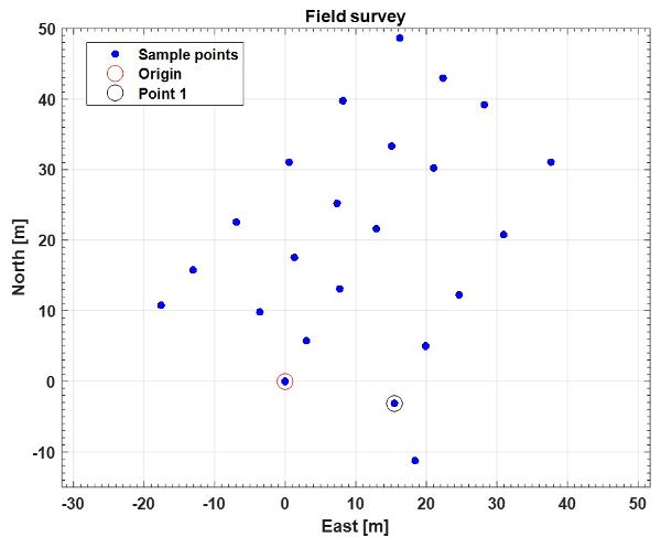
A soil-surveying robot uses a GPS receiver to locate sampling points forming a grid in a field. Those points constitute the reference base for several precision farming applications related to the spatial distribution of soil properties such as compactness, pH, and moisture content. The location data (Table 3.4.2) provided by the GPS receiver is in a standard NMEA code format. Transform the data (i.e., the geodetic coordinates provided by a handheld GPS receiver) to the local tangent plane (LTP) frame to be more directly useful to farmers.
Solution
The first step in the transformation process requires the selection of a reference ellipsoid. Choose the WGS 84 reference ellipsoid because it is widely used for agricultural applications. Use Equations 3.4.2 to 3.4.7 and apply the transform function (Equation 3.4.8) to the 23 points given in geodetic coordinates (Table 3.4.2) to convert them into LTP coordinates. For that reference ellipsoid,
\( a = \text{semi-major axis of WGS 84 reference ellipsion} = 6378137\ m \)
\( e = \text{eccentricity of WGS 84 reference ellipsion} = 0.0818 \)
\( N_{0}(\lambda) = \frac{a}{\sqrt{1-e^{2} \cdot sin^{2}\lambda}} \) (Equation \(\PageIndex{4}\))
\( (N_{0}+h) \cdot cos\lambda \cdot cos\phi \) (Equation \(\PageIndex{5}\))
\( Y= (N_{0}+h) \cdot cos\lambda \cdot sin\phi \) (Equation \(\PageIndex{6}\))
\( Z = [h+N_{0} \cdot (1-e^{2})] \cdot sin\lambda \) (Equation \(\PageIndex{7}\))
\( \begin{bmatrix} N \\E\\D \end{bmatrix} = \begin{bmatrix} -sin \lambda \cdot cos\phi & -sin\lambda \cdot sin\phi & cos\lambda \\ -sin\phi &cos\phi & 0 \\ -cos\lambda \cdot cos\phi & -cos\lambda \cdot sin\phi & -sin\lambda \end{bmatrix} \cdot \begin{bmatrix} X-X_{0} \\ Y-Y_{0} \\ Z-Z_{0} \end{bmatrix} \) (Equation \(\PageIndex{8}\))
The length of the normal N0 is the distance from the surface of the ellipsoid of reference to its intersection with the rotation axis and [λ, φ, h] is a point in geodetic coordinates recorded by the GPS receiver; [X, Y, Z] is the point transformed to ECEF coordinates (m), with [X0, Y0, Z0] being the user-defined origin of coordinates in ECEF; and [N, E, D] is the point being converted in LTP coordinates (m).
| Point | Latitude (°) | Latitude (min) | Longitude (°) | Longitude (min) | Altitude (m) |
|---|---|---|---|---|---|
|
Origin |
39 |
28.9761 |
0 |
−20.2647 |
4.2 |
|
1 |
39 |
28.9744 |
0 |
−20.2539 |
5.1 |
|
2 |
39 |
28.9788 |
0 |
−20.2508 |
5.3 |
|
3 |
39 |
28.9827 |
0 |
−20.2475 |
5.9 |
|
4 |
39 |
28.9873 |
0 |
−20.2431 |
5.6 |
|
5 |
39 |
28.9929 |
0 |
−20.2384 |
4.8 |
|
6 |
39 |
28.9973 |
0 |
−20.2450 |
5.0 |
|
7 |
39 |
28.9924 |
0 |
−20.2500 |
5.2 |
|
8 |
39 |
28.9878 |
0 |
−20.2557 |
5.2 |
|
9 |
39 |
28.9832 |
0 |
−20.2593 |
5.4 |
|
10 |
39 |
28.9792 |
0 |
−20.2626 |
5.2 |
|
11 |
39 |
28.9814 |
0 |
−20.2672 |
4.8 |
|
12 |
39 |
28.9856 |
0 |
−20.2638 |
5.5 |
|
13 |
39 |
28.9897 |
0 |
−20.2596 |
5.5 |
|
14 |
39 |
28.9941 |
0 |
−20.2542 |
5.0 |
|
15 |
39 |
28.9993 |
0 |
−20.2491 |
5.0 |
|
16 |
39 |
29.0024 |
0 |
−20.2534 |
5.1 |
|
17 |
39 |
28.9976 |
0 |
−20.2590 |
4.9 |
|
18 |
39 |
28.9929 |
0 |
−20.2643 |
4.9 |
|
19 |
39 |
28.9883 |
0 |
−20.2695 |
4.9 |
|
20 |
39 |
28.9846 |
0 |
−20.2738 |
4.8 |
|
21 |
39 |
28.9819 |
0 |
−20.2770 |
4.7 |
|
22 |
39 |
28.9700 |
0 |
−20.2519 |
4.5 |
MATLAB® can provide a convenient programming environment to transform the geodetic coordinates to a flat frame, and save them in a text file. Table 3.4.3 summarizes the results as they would appear in a MATLAB® (.m) file.
These 23 survey points can be plotted in a Cartesian frame East-North (namely in LTP coordinates) to see their spatial distribution in the field, with East and North axes oriented as shown in Figure 3.4.10.
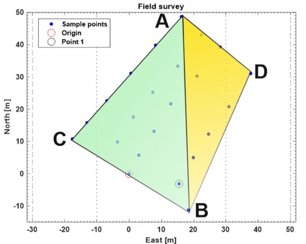
A crucial advantage of using flat coordinates like LTP is that Euclidean geometry can be extensively used to calculate distances, areas, and volumes. For example, to calculate the total area covered by the surveyed grid, split the resulting trapezoid into two irregular triangles (Figure 3.4.11), one defined by the points A-B-C, and the other by the three points A-B-D. Apply Euclidean geometry to calculate the area of an irregular triangle from the measurement of its three sides using the equation:
| Point | East (m) | North (m) | Down (m) |
|---|---|---|---|
|
Origin |
0 |
0 |
0 |
|
1 |
15.5 |
−3.1 |
−0.9 |
|
2 |
19.9 |
5.0 |
−1.1 |
|
3 |
24.7 |
12.2 |
−1.7 |
|
4 |
31.0 |
20.7 |
−1.4 |
|
5 |
37.7 |
31.1 |
−0.6 |
|
6 |
28.2 |
39.2 |
−0.8 |
|
7 |
21.1 |
30.2 |
−1.0 |
|
8 |
12.9 |
21.6 |
−1.0 |
|
9 |
7.7 |
13.1 |
−1.2 |
|
10 |
3.0 |
5.7 |
−1.0 |
|
11 |
−3.6 |
9.8 |
−0.6 |
|
12 |
1.3 |
17.6 |
−1.3 |
|
13 |
7.3 |
25.2 |
−1.3 |
|
14 |
15.1 |
33.3 |
−0.8 |
|
15 |
22.4 |
42.9 |
−0.8 |
|
16 |
16.2 |
48.7 |
−0.9 |
|
17 |
8.2 |
39.8 |
−0.7 |
|
18 |
0.6 |
31.1 |
−0.7 |
|
19 |
−6.9 |
22.6 |
−0.7 |
|
20 |
−13.0 |
15.7 |
−0.6 |
|
21 |
−17.6 |
10.7 |
−0.5 |
|
22 |
18.3 |
−11.3 |
−0.3 |
\( \text{Area} = \sqrt{K \cdot (K-a) \cdot (K-b)\cdot (K-c)} \) (Equation \(\PageIndex{14}\))
where, a, b, and c are the lengths of the three sides of the triangle, and \( K=\frac{a+b+c}{2} \).
The distance between two points A and B can also be determined by the following equation:
\( L_{A-B} = \sqrt{(E_{A}-E_{B})^{2} +(N_{A}-N_{B})^{2}} \) (Equation \(\PageIndex{15}\))
where LA-B = Euclidean distance (straight line) between points A and B (m)
[EA, NA] = the LTP coordinates east and north of point A (m)
[EB, NB] = the LTP coordinates east and north of point B (m), calculated in Table 3.4.3.
Using the area equation, the areas of the two triangles presented in Figure 3.4.11 are determined as 627 m2 for the yellow triangle (ADB) and 1,054 m2 for the green triangle (ABC), with a total area of 1,681 m2. The corresponding Euclidean distances are 50.9 m, 42.1 m, 60.0 m, 27.8 m, and 46.6 m, respectively, for LA-C, LC-B, LA-B, LA-D, and LD-B, as:
\( L_{A-B} = \sqrt{(E_{A}-E_{B})^{2} +(N_{A}-N_{B})^{2}}=\sqrt{(16.2-18.3)^{2} +(48.7-(-11.3))^{2}} = 60.0 \)
We have not said anything about the Z direction of the field, but the Altitude column in Table 3.4.2 and the Down column in Table 3.4.3 both suggest that the field is quite flat, as the elevation of the points over the ground does not vary by much along the 22 points.
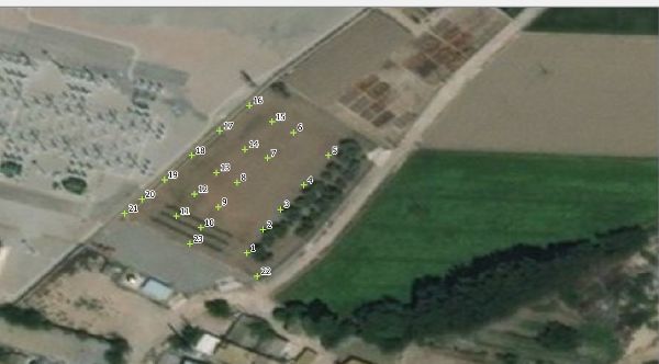
Figure 3.4.12 shows the sampled points of Figure 3.4.10 overlaid with a satellite image that allows users to know additional details of the field such as crop type, lanes, surrounding buildings (affecting GPS performance), and other relevant information.
Example \(\PageIndex{3}\)
Example 3: Configuration of a machine vision system for detecting cherry tomatoes on an intelligent harvester
Problem:
Assume you are involved in designing an in-field quality system for the on-the-fly inspection of produce on board an intelligent cherry tomato harvester. Your specific assignment is the design of a machine vision system to detect blemishes in cherry tomatoes being transported by a conveyor belt on the harvester, as illustrated in Figure 3.4.13. You are required to use an existing camera that carries a CCD sensor of dimensions 6.4 mm × 4.8 mm. The space allowed to mount the camera (camera height h) is about 40 cm above the belt. However, you can buy any lens to assure a horizontal FOV of 54 cm to cover the entire width of the conveyor belt. Determine the required focal length of the lens.
Solution
The first step in the design of this sensing system is to calculate the focal length (f) of the lens needed to cover the requested FOV. Normally, the calculation of the focal length requires knowing two main parameters of lens geometry: the distance between the CCD sensor and the optical center of the lens, d1, and the distance between the optical center of the lens and the conveyor belt, d2. We know d2 = 400 mm, FOV = 540 mm, and A, the horizontal dimension of the imaging sensor, is 6.4 mm, so d1 can be easily determined according to Equations 3.4.10 and 3.4.11:
\( \frac{d_{1}}{d_{2}} = \frac{A}{FOV} \) (Equation \(\PageIndex{11}\))
Thus,
\( d_{1} = \frac{A \cdot d_{2}}{FOV} = \frac{6.4 \cdot 400}{540} = 4.74 \ mm \)
The focal length, f, can then be determined using Equation 3.4.10:
\( \frac{1}{f} = \frac{1}{d_{1}} + \frac{1}{d_{2}} \) (Equation \(\PageIndex{10}\))
Thus,
\( f= \frac{d_{1} \cdot d_{2}}{d_{1} + d_{2}} = \frac{4.74 \cdot 400}{4.74 + 400} = 4.68 \ mm \)
No lens manufacturer will likely offer a lens with a focal length of 4.68 mm; therefore, you must choose the closest one from what is commercially available. The lenses commercially available for this camera have the following focal lengths: 2.8 mm, 4 mm, 6 mm, 8 mm, 12 mm, and 16 mm. A proper approach is to choose the best lens for this application, and readjust the distance between the camera and the belt in order to keep the requested FOV covered. Out of the list offered above, the best option is choosing a lens with f = 4 mm. That choice will change the original parameters slightly, and you will have to readjust some of the initial conditions in order to maintain the same FOV, which is the main condition to meet. The easiest modification will be lowering the position of the camera to a distance of 34 cm to the conveyor (d2 = 340 mm from the focal length equation). If the camera is fixed and d2 has to remain at the initial 40 cm, the resulting field of view would be larger than the necessary 54 cm, and applying image processing techniques would be necessary to remove useless sections of the images.
Example \(\PageIndex{4}\)
Example 4: Estimation of a robot velocity using an accelerometer
Problem:
| Data point | Time (s) | Acceleration (g) |
|---|---|---|
|
1 |
7.088 |
0.005 |
|
2 |
8.025 |
0.018 |
|
3 |
9.025 |
0.009 |
|
4 |
10.025 |
0.009 |
|
5 |
11.025 |
0.008 |
|
6 |
12.025 |
0.009 |
|
7 |
13.025 |
0.009 |
|
8 |
14.025 |
0.009 |
|
9 |
15.025 |
0.008 |
|
10 |
16.025 |
0.008 |
|
11 |
17.025 |
0.009 |
|
12 |
18.025 |
0.009 |
|
13 |
19.025 |
0.008 |
|
14 |
20.088 |
0.009 |
|
15 |
21.088 |
−0.009 |
|
16 |
21.963 |
−0.019 |
|
17 |
23.025 |
−0.001 |
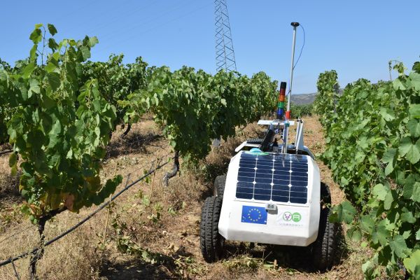
The accelerometer of Figure 3.4.14a was installed in the agricultural robot of Figure 3.4.14c. When moving along vineyard rows, the output measurements from the accelerometer were recorded in Table 3.4.4, including the time of each measurement and its corresponding linear acceleration in the forward direction given in g, the gravitational acceleration.
- 1. Calculate the instantaneous acceleration of each point in m·s−2, taking into account that one g is equivalent to 9.8 m·s−2.
- 2. Calculate the time elapsed between consecutive measurements ∆t in s.
- 3. Estimate the average sample rate (Hz) at which the accelerometer was working.
- 4. Calculate the corresponding velocity for every measurement with Equation 3.4.12, taking into account that the vehicle started from a resting position (V0 = 0 m s−1) and always moved forward.
- 5. Plot the robot’s acceleration (m s−2) and velocity (km h−1) for the duration of the testing run.
(a)
(b)
(c)
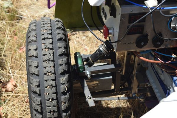
Figure \(\PageIndex{14}\): (a) Accelerometer Gulf Coast X2-2; (b) sensor mounting; (c) in an agricultural robot.
Solution
| Data point | Time (s) | Acceleration (g) | Acceleration (m s−2) | ∆t (s) |
|---|---|---|---|---|
|
1 |
7.088 |
0.005 |
0.050 |
0 |
|
2 |
8.025 |
0.018 |
0.179 |
0.938 |
|
3 |
9.025 |
0.009 |
0.091 |
1.000 |
|
4 |
10.025 |
0.009 |
0.085 |
1.000 |
|
5 |
11.025 |
0.008 |
0.083 |
1.000 |
|
6 |
12.025 |
0.009 |
0.088 |
1.000 |
|
7 |
13.025 |
0.009 |
0.085 |
1.000 |
|
8 |
14.025 |
0.009 |
0.084 |
1.000 |
|
9 |
15.025 |
0.008 |
0.080 |
1.000 |
|
10 |
16.025 |
0.008 |
0.081 |
1.000 |
|
11 |
17.025 |
0.009 |
0.086 |
1.000 |
|
12 |
18.025 |
0.009 |
0.084 |
1.000 |
|
13 |
19.025 |
0.008 |
0.083 |
1.000 |
|
14 |
20.088 |
0.009 |
0.089 |
1.063 |
|
15 |
21.088 |
−0.009 |
−0.092 |
1.000 |
|
16 |
21.963 |
−0.019 |
−0.187 |
0.875 |
|
17 |
23.025 |
−0.001 |
−0.009 |
1.063 |
|
Average |
0.996 |
|||
According to the previous results, the average time elapsed between two consecutive measurements ∆t is 0.996 s, which corresponds to approximately one measurement per second, or 1 Hz. The velocity of a vehicle can be estimated from its acceleration with Equation 3.4.12. Table 3.4.5 specifies the calculation at each specific measurement.
Figure 3.4.15 plots the measured acceleration and the calculated velocity for a given time interval of 16 seconds. Notice that there are data points with a negative acceleration (deceleration) but the velocity is never negative because the vehicle always moved forward or stayed at rest. Accelerometers suffer from noisy estimates, and as a result, the final velocity calculated in Table 3.4.5 may not be very accurate. Consequently, it is a good practice to estimate vehicle speeds redundantly with at least two independent sensors working under different principles. In this example, for instance, forward velocity was also estimated with an onboard GPS receiver.
| Data point | Acceleration (m s−2) | ∆t (s) | Velocity (m s−1) | V (km h−1) |
|---|---|---|---|---|
|
1 |
0.050 |
0 |
V1 = V0 + a1 · ∆t = 0 + 0.05 · 0 = 0 |
0.0 |
|
2 |
0.179 |
0.938 |
V2 = V1 + a2 · ∆t = 0 + 0.179 · 0.938 = 0.17 |
0.6 |
|
3 |
0.091 |
1.000 |
V3 = V2 + a3 · ∆t = 0.17 + 0.091 · 1 = 0.26 |
0.9 |
|
4 |
0.085 |
1.000 |
0.34 |
1.2 |
|
5 |
0.083 |
1.000 |
0.43 |
1.5 |
|
6 |
0.088 |
1.000 |
0.51 |
1.9 |
|
7 |
0.085 |
1.000 |
0.60 |
2.2 |
|
8 |
0.084 |
1.000 |
0.68 |
2.5 |
|
9 |
0.080 |
1.000 |
0.76 |
2.7 |
|
10 |
0.081 |
1.000 |
0.84 |
3.0 |
|
11 |
0.086 |
1.000 |
0.93 |
3.3 |
|
12 |
0.084 |
1.000 |
1.01 |
3.7 |
|
13 |
0.083 |
1.000 |
1.10 |
3.9 |
|
14 |
0.089 |
1.063 |
1.19 |
4.3 |
|
15 |
-0.092 |
1.000 |
1.10 |
4.0 |
|
16 |
-0.187 |
0.875 |
0.94 |
3.4 |
|
17 |
-0.009 |
1.063 |
0.93 |
3.3 |
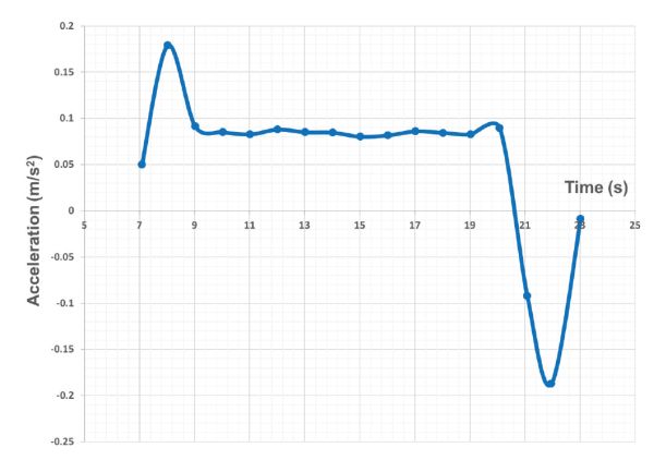
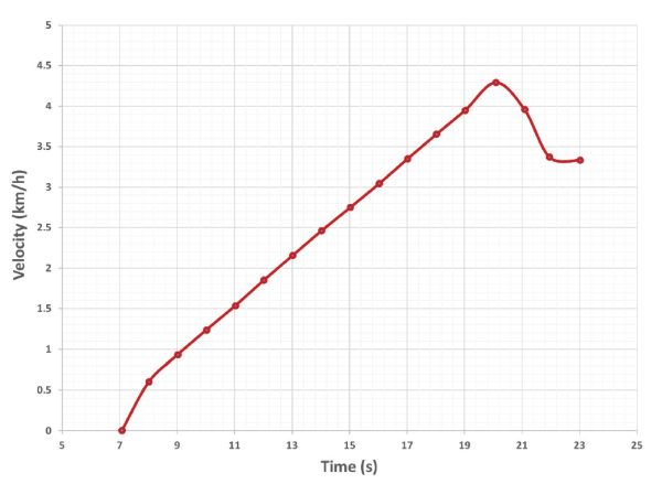
Image Credits
Figure 1a. John Deere. (2020). Autonomous mower. Retrieved from www.deere.es/es/campaigns/ag-turf/tango/. [Fair Use].
Figure 1b. Rovira-Más, F. (CC BY 4.0). (2020). (b) GPS-based autonomous rice transplanter.
Figure 2. Verified Market Research (2018). (CC BY 4.0). (2020). Expected growth of agricultural robot market.
Figure 3. Rovira-Más, F. (CC BY 4.0). (2020). Sensor architecture for intelligent agricultural vehicles.
Figure 4. Rovira-Más, F. (CC BY 4.0). (2020). Geometrical relationship between an imaging sensor, lens, and FOV.
Figure 5. Rovira-Más, F. (CC BY 4.0). (2020). Color-based segmentation of mandarin oranges.
Figure 6. Rovira-Más, F. (CC BY 4.0). (2020). Auto-guidance systems: (a) Light-bar kit; (b) Parallel tracking control screen.
Figure 7. Zhang, Q. (CC BY 4.0). (2020). Tractor steering systems: (a) traditional hydraulic steering system; and (b) electrohydraulic steering system.
Figure 8. Adapted from T. Karvinen, K. Karvinen, V. Valtokari (Make: Sensors, Maker Media, 2014). (2020). Assembly of an ultrasonic rangefinder HC-SR04 with an Arduino processor. [Fair Use].
Figure 9. Rovira-Más, F. (CC BY 4.0). (2020). Digitalization of an analog signal with 4 bits between 1.2 V and 4.7 V.
Figure 10. Rovira-Más, F. (CC BY 4.0). (2020). Planar representation of the 23 points sampled in the field with a local origin.
Figure 11. Rovira-Más, F. (CC BY 4.0). (2020). Estimation of the area covered by the sampled points in the surveyed field.
Figure 12. Saiz-Rubio, V. (CC BY 4.0). (2020). Sampled points over a satellite image of the surveyed plot (origin in number 23).
Figure 13. Rovira-Más, F. (CC BY 4.0). (2020). Geometrical requirements of a vision-based inspection system for a conveyor belt on a harvester.
Figure 14a. Gulf Coast Data Concepts. (2020). Accelerometer Gulf Coast X2-2. Retrieved from http://www.gcdataconcepts.com/x2-1.html. [Fair Use].
Figure 14b & 14c. Saiz-Rubio, V. (CC BY 4.0). (2020). (b) sensor mounting. (c) mounting an agricultural robot.
Figure 15. Rovira-Más, F. (CC BY 4.0). (2020). Acceleration and velocity of a farm robot estimated with an accelerometer.
References
Bolton, W. (1999). Mechatronics (2nd ed). New York: Addison Wesley Longman Publishing.
Myklevy, M., Doherty, P., & Makower, J. (2016). The new grand strategy. New York: St. Martin’s Press.
Rovira-Más, F., Zhang, Q., & Hansen, A. C. (2010). Mechatronics and intelligent systems for off-road vehicles. London: Springer-Verlag.
Russell, S., & Norvig, P. (2003). Artificial Intelligence: a modern approach (2nd ed). Upper Saddle River, NJ: Prentice Hall.
Verified Market Research. (2018). Global agriculture robots market size by type (driverless tractors, automated harvesting machine, others), by application (field farming, dairy management, indoor farming, others), by geography scope and forecast. Report ID: 3426. Verified Market Research Inc.: Boonton, NJ, USA, pp. 78.