
3.2: Crop Establishment and Protection
- Page ID
- 46846

Roberto Oberti
Department of Agricultural and Environmental Science, University of Milano, Milano, Italy
Peter Schulze Lammers
Department of Agricultural Engineering, University of Bonn, Bonn, Germany
| Key Terms |
| Tillage | Spreading | Field performance parameters |
| Planting | Spraying | Application rate and quality |
Variables
Introduction
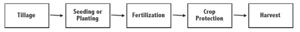
Field crops are most often grown to provide food for humans and for animals. Growing field crops requires a sequence of operations (Figure 3.2.1) that usually starts with land preparation followed by planting. These two stages are known as crop establishment. Crop growth requires a supply of nutrients through application of fertilizers as well as protection against weeds, diseases, and pest insects using biological, chemical, and/or physical treatments. Finally, the crop is harvested and transported to processing locations. This general sequence of operations can be more complex or specifically modified for a particular crop or cropping system. For example, crop establishment is only required once, while crop protection and fertilization may be repeated multiple times annually.
Engineering is integral to maximize the productivity and efficiency of these operations. This chapter introduces some of the engineering concepts and equipment used for crop establishment and crop protection in arable agriculture.
Outcomes
After reading this chapter, you should be able to:
- Describe the fundamental principles of agricultural mechanization
- Apply physics concepts to some aspects of crop establishment and protection equipment
- Calculate field performance for land preparation, planting, fertilizing, and plant protection based on operating parameters
Concepts
Field Performance Parameters
Regardless of the specific operation, the work of a field machine is evaluated through some fundamental parameters: the operating width and the field capacity of the machine.
Operating Width
The operating, or working, width w of a machine is the width of the portion of field worked by each pass of the machine. In field work, especially with large equipment, the effective operating width can be less than the theoretical width due to unwanted partial overlaps between passes.
Field Capacity of a Machine
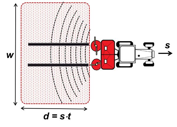
An important parameter to be considered when selecting a machine for an operation is the field capacity, which represents the machine’s work rate in terms of area of land or crop processed per hour. The theoretical field capacity of the machine (also called the area capacity) can be computed as:
\[ c_{t} = ws \]
where Ct = theoretical field capacity (m2 h−1)
w = operating width (m)
s = field speed (m h−1)
Ct is typically expressed in ha h−1. Figure 2 illustrates the field area worked during a time interval, t.
In actual working conditions, this theoretical capacity is reduced by idle times (e.g., turnings, refills, transfers, or breaks) and possible reductions in working width or in nominal field speed due to operational considerations, resulting in an actual field capacity:
\[ c_{a} = e_{f}C_{t} \]
where ef is the field efficiency (decimal). Its value largely depends on the operation, which can be estimated for given operations and working conditions.
Tillage
Definition of Tillage
Soil preparation by mechanical interventions is called tillage. The major function of tillage is loosening the soil to create pores so they can contain air and water to enable the growth of roots. Other main tasks of tillage are crushing soil aggregates to required sizes, reduction or elimination of weeds, and admixing of plant residues. Tillage needs to be adapted to the soil type and condition (such as soil water or plant residue content) and conducted at a proper time.
Soil Mechanics
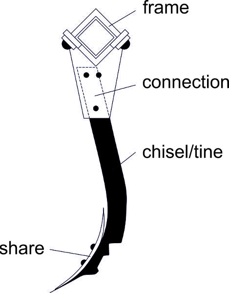
Soil is classified by grain sizes into sand, silt, and clay categories. Loam is a mixture of these soil types. Soil is subjected to shear stress and reacts by strain when it is tilled. The tillage tool moving through the soil causes a force which causes a stress between adjacent soil grains. This leads to a deformation or strain of the soil. Sandy soil is characterized by low shear strength and high friction, while clay is characterized by high cohesion and, after cracking, by low friction. Tillage tools usually act as wedges. They engage with the soil and cause relative movement in a shear plane where some of the soil moves with the tool while the adjacent soil stays in place. Energy is expended in shearing and lifting of the soil and overcoming the friction on the tool.
Primary Tillage
Primary tillage tools or implements are designed for loosening the soil and mixing or incorporating crop residues left on the field surface after harvest. Subsequent soil treatment to prepare a seedbed is secondary tillage. A typical implement for primary tillage is the plow (spelled “plough” in some countries), which is used for deep soil cultivation.
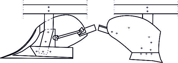
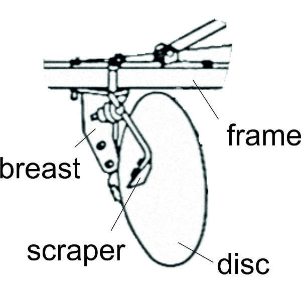
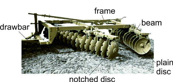
The three most common kinds of plow are moldboard, chisel, and disc (Figure 3.2.3). The moldboard plow body and its action are shown in Figure 3.2.3a. A plow share cuts the soil horizontally and the attached moldboard upturns the soil strip and turns it almost upside down in the furrow made by the previous plow body. The heel makes sure the plow follows the proper path. These parts are connected by a supporting part (breast) which is connected by a leg to the frame of the plow. Chisel plows do not invert all the soil, but they mix the top soil layer, including residues, into deeper portions of the soil. Chisel plows use heavy tines with shares on the bottom of the tines (Figure 3.2.3b). A disc plow uses concave round discs (Figure 3.2.3c) to cut the soil on the furrow bottom and turns the soil with the rotating motion of the disc.
The draft forces to pull a plow are provided by a tractor to which it is attached. Equation 3.2.3 is one way used to calculate the draft force needed to pull a moldboard plow. This calculation follows Gorjachkin (1968):
\[ F_{z} = nF_{v} \rho_{r} + ikw_{f}d \ + i \epsilon w_{f} dv^{2} \]
where Fz = draft force (N)
n = number of gauge wheels
Fv = vertical force (N)
ρR = rolling resistance
i = number of moldboards or shares
k = static factor (N cm−2) ranging from 2 to 14 depending on soil type
wf = width of furrow (cm)
d = depth of furrow (cm)
ε = dynamic factor (N s2 m−2 cm−2), ranging from 0.15 to 0.36 depending on soil type and moldboard design
v = traveling speed (m s−1)
About half the energy consumed in plowing, the effective energy, does the work of cutting (13–20%), elevating and accelerating the soil (13–14%), and deformation (14–15%). The remaining energy is spent on noneffective losses (e.g., friction), which do not contribute to tillage effectiveness.
Secondary Tillage (Seedbed Preparation)
Secondary tillage prepares the seedbed after primary tillage. Implements for secondary tillage are numerous and of many different designs. A harrow is the archetype of secondary tillage; it consists of tines fixed in a frame. Cultivators are heavier, with longer tines formed as chisels in a rigid frame or with a flexible suspension. Soil is opened by shares and the effect is characterized by the tine spacing, depth of furrow, and speed.
(a)
(b)
(c)
Figure \(\PageIndex{3}\): (a) moldboard plow body; (b) chisel (tine) of a cultivator; (c) disc plow.
Most tillage implements are pulled by tractors and limited by traction, as discussed in another chapter. (Power tillers exist as rotary harrows with vertical axles or rotary cultivators with horizontal axles; these are discussed below.) The mechanical connection of the tractor power take-off (PTO) to the tillage implement provides the power to drive the implement’s axles, which are equipped with blades, knives, or shares. Each blade cuts a piece of soil (Schilling, 1962) and the length of that bite is determined as a function of the tractor travel speed and axle rotation speed according to:
\[ B= \frac{\nu\ 10,000}{rz\ 60} \]
where B = bite length (cm)
v = travel speed (km h−1)
r = rotary speed (min−1)
z = number of blades per tool assembly
The cut soil is often flung against a hood or cover which helps crush soil agglomerations, with the axle rotation speed affecting the impact force.
Planting
Crops are sown (planted) by placing seeds in the soil (or in some cases, discussed below, by transplanting). Basic requirements are:
- • equal distribution of seeds in the field,
- • placing the seeds at the proper depth of soil, and
- • covering the seeds.
The seed bed should be prepared by tilling the soil to aggregates the size of the seed grain, and gently compacting the soil at the placement depth of the seed, e.g., 2–4 cm for wheat and barley. Germination is triggered by soil temperature (e.g., 2–4°C for wheat) and soil water content. The seeding rate of cereal grains is in the range of 200 to 400 grains per m2 resulting in 500 to 900 heads per m2 as a single plant may produce multiple heads. As the metering of seeds is mass-based, commercial seed is indexed by the mass of one thousand grains (Table 3.2.1).
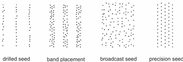
The appropriate distribution of seeds is a fundamental condition for a successful crop yield. Seeds can be broadcasted, which means they are scattered randomly (Figure 3.2.4). This is commonly done for crops such as grasses and alfalfa. But the seeds for most crops are deposited in rows. Common distances between rows for cereals are 12 to 15 cm. For crops commonly called row crops (e.g., soybean or maize), the row spacing is 45 to 90 cm. If the rows are at a suitable distance, the wheels of farm machines can avoid driving on the plants as they grow from the seeds.
| Thousand Grain Mass (g) |
Bulk Density (kg L−1) |
Seed Rate (kg ha−1) |
Area per Grain (cm2) |
|
|---|---|---|---|---|
|
Wheat (Triticum aestivum) |
25–50 |
0.76 |
100–250 |
22–37 |
|
Barley (Hordeum vulgare) |
24–48 |
0.64 |
100–180 |
27–48 |
|
Maize (Zea mays) |
100–450 |
0.7 |
50–80 |
- |
|
Peas (Pisum sativum) |
78–560 |
0.79 |
120–280 |
- |
|
Rapeseed (Brassica napus) |
3.5–7 |
0.65 |
6–12 |
- |
Within rows, seeds have a random spacing if seed drills are used, or have a fixed distance between seeds if precision seeders (discussed below) are used. Seed drills are commonly used for small grains and consist of components that:
- • hold the seeds to be planted,
- • meter (singulate) the seed,
- • open a row furrow in the soil,
- • transport the seeds to the soil,
- • place the seeds in the soil, and then
- • cover the open furrow with soil.
To extend the area per seed when sowing in rows, a wider opening of the furrow allows band seeding (Figure 3.2.4).
(a)
(b)
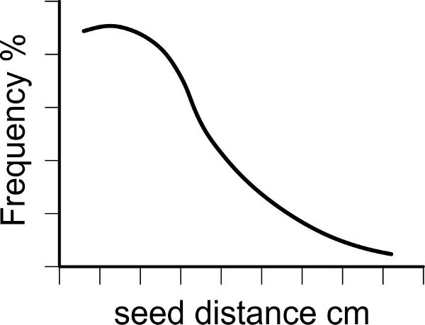
Figure \(\PageIndex{6}\): (a) Seed deposition in a row, drilled; (b) frequency of seed distances, drilled.
Regular seed drills often meter the seeds with a studded roller as seen in Figure 3.2.5. The ideal is to have a uniform distribution, but there will be variation, including infrequent longer distances, as shown by Figure 3.2.6 (Heege, 1993).
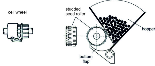
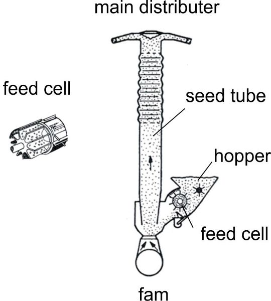
A second very common metering device is a cell wheel, which is used for central metering in pneumatic seed drills. A rotating cell wheel is filled by the seeds in the hopper and empties into an air stream via a venturi jet (Figure 3.2.7). The grains are entrained by air and collide with a plate. A relatively uniform distribution of grains occurs along the circumference of the plate where pipes for transporting the grains to the coulters are arranged.
The frequency of the seed distances (Figure 3.2.6) as metered by the feed cells or studded rollers corresponds to an exponential function (Heege, 1993):
\[ p_{z} = \frac{1}{\bar{x}}e^{-\frac{x_{i}}{\bar{x}}} \]
where pz = seed spacing frequency
xi = seed spacing (cm)
\(\bar{x}\) = mean seed spacing (cm)
The accuracy of the longitudinal seed distribution is indicated by the coefficient of variation (Müeller et al., 1994):
\[ CV= \frac{\sqrt{\frac{(x_{i} - \bar{x})^{2}}{N-1}}}{\bar{x}} 100\% \]
where CV = coefficient of variation (%)
N = number of measured samples
xi = spacing (cm)
\(\bar{x}\) = mean spacing (cm)
A CV smaller than 10% is considered good, while above 15% is unsatisfactory.
Precision Seed Drills
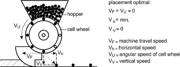
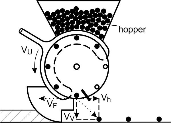
Crops such as maize, soybeans, sugar beets, and cotton have higher yields if seeded as single plants. Precision seed drills singulate the seeds and place them at constant separation distances in the row. Cell wheels single the seeds out of the bulk, move them by constant rotational speed to the coulter, and drop them in the seed furrow with a target distance between each seed. Filling of the cells is a crucial function of precision seed drills. Every cell needs to be filled with one, and only one, seed. The cell wheels rotate through the bulk of seeds in the hopper and are filled by gravity, or the filling is accomplished by an air stream sucking the grains to the holes of the cell wheels (Figure 3.2.8). Then the seeds are released from the cell wheels and drop onto the bottom of the seed furrow. The trajectory of a single seed grain is affected by gravity (including the time for the seed to drop). To avoid rolling of the seeds in the furrow, the backward speed of the seed relative to the drill should match the forward speed of the seed drill.
The time required for the seed to drop is:
\[ t= \sqrt{\frac{2h}{g}} \]
where t = time of dropping (s)
h = height of cell above seed furrow (m)
g = acceleration due to gravity (9.8 m s−2)
(a)
(b)
Figure \(\PageIndex{8}\): Precision seeder singling seed grains for seed placement with definite spacing: (a) mechanical singling by cell wheel, (b) pneumatic singling device with cell wheel.
Transplanting
In the case of short vegetation periods or intensive agriculture (e.g., crops that require production in a short time), some crops are not direct-seeded into fields but instead are transplanted.
Seeds may be germinated under controlled conditions, such as in greenhouses (glasshouses). The small plant seedlings may be grown on trays or in pots then transplanted into fields where they will produce a harvestable crop. In the case of rice, which is often not direct-seeded, the plants are grown in trays and then transplanted. When transplanting rice, an articulated mechanical device punches the root portion together with the upper parts of the plants out of the tray and presses it into the soil, while keeping the plants fully saturated with water.
Other plants are propagated by vegetative methods (cloning or cuttings). Special techniques are required for potatoes. “Seed” tubers are put in the hopper of the planter and planted in ridges. Row distances are commonly 60–90 cm, which produce 40,000–50,000 potatoes per ha.
Compared to seeds, small plants (whether seedlings, tubers, cuttings, etc.) are easily damaged. The fundamental requirements of transplanting, both manual (which is labor-intensive) and mechanized, are:
- • no damage to the seedlings,
- • upright positioning of the seedlings in the soil at a target depth,
- • correct spacing between plants in a row, and
- • close contact of the soil with the roots.
Fertilization
Crop yield is strictly related to the availability of nutrients that are absorbed by the plant during growth. As crops are harvested, nutrients are removed from the soils. The major nutrients (nitrogen (N), phosphorus (P), and potassium (K)) usually have to be replaced by the application of fertilizers in order to maintain the soil’s productivity. Minor nutrients are also sometimes needed.
Organic fertilizers are produced within the farming process, and their use can be seen as a conservation recycling of nutrients. The concentration of nutrient elements in organic fertilizers is low (e.g., 1 kg of livestock slurry can contain 5 g of N or less), requiring very large structures for long-term storage, suitable protection from nutrient volatilization or dilution, large machines for field distribution, and the application of large amounts for sufficient fertilization of crops. Based on their solid contents, organic fertilizers are classified as slurry (solid content less than 14%) that can be pumped and managed as fluids, or as manure (solid content at least 14%) that are managed as solids with scrapers and forks.
Mineral fertilizers are produced by industrial processes and are characterized by a high concentration of nutrient chemicals, prompt availability for plant uptake, ease of storage and handling, and stability over time. The most used form of mineral fertilizers worldwide is solid granules (e.g., urea prills, calcium ammonium nitrate, potassium chloride, and N-P-K compound fertilizers). Other techniques rely on the distribution of liquid solutions or suspensions of mineral fertilizers or on soil injection of anhydrous ammonia.
Application Rate
During distribution operations (including fertilization as well as distribution of other inputs such as pesticides), the application rate is the amount of material distributed per unit of surface area, i.e., for solids by mass:
\[ AR=M/A \]
and for liquids by volume:
\[ AR=V/A \]
where AR = application rate (kg ha−1 or L ha−1)
M = mass of material distributed (kg)
V = volume of material distributed (L)
A = field area receiving the material (ha)
Dose of Application
The dose of application, D, refers to the amount of active compound (e.g., chemical nutrient, pesticide ingredient) distributed per unit of surface area:
\[ D=c_{AC}AR \]
where D = dose of application (kgAC ha−1)
cAC = content of active compound in the raw material or solution distributed at the application rate (g kg−1 or g L−1)
Longitudinal and Lateral Uniformity of Distribution
The uniformity of the application rate during distribution is of fundamental importance for the agronomic success of the operation. The machine must be able to guarantee a suitable uniformity along both the traveling (longitudinal uniformity) and the transversal (lateral uniformity) directions.
The longitudinal uniformity of the distribution to the field is obtained by appropriate metering of the mass (or volume) flow out of the machine, by means of control devices such as adjustable discharge gates or valves. The rate of material flow to be set depends on the desired application rate, the traveling speed, and the working width of the distributing machine. This can be seen by dividing by time both the numerator and denominator of Equation 3.2.8 (and similarly for 3.2.9), which leads to:
\( AR = (M/t)/(A/t) \)
The numerator of the right side of the equation is the mass outflow Q (typically expressed in kg min−1), and the denominator is the theoretical field capacity of the machine Ct, or 0.1 w s (see Equation 3.2.1).
Then, it follows that, for AR in units of kg ha−1:
\( AR = \frac{(Q \text{ kg min}^{-1}) (60 \text{ min h}^{-1})}{0.1 ws} = \frac{600Q}{ws} \)
Rearranging:
\[ Q= \frac{AR \ ws}{600} \]
where Q is the value of material flow (kg min−1) to be set in order to obtain a desired application rate AR (kg ha−1), when the distributing machine works at a speed s (km h−1) and with a working width w (m).
Similarly, for liquid material distributed, the volume rate q (L min−1) is calculated as follows:
\[ q= \frac{AR \ ws}{600} \]
The lateral uniformity of distribution along the working width is obtained by ensuring two conditions: a controlled distribution pattern and an appropriate overlapping of swath distance between the adjacent passes of machine. A properly operating distribution system can maintain the regular shape of the distribution pattern, which can be triangular, trapezoidal, or rectangular, depending on the distribution system. The overall lateral distribution is obtained by the proper overlapping of the individual pattern produced by each pass of the equipment (the working width). The uniformity of distribution can be tested by travelling past trays placed on the ground and measuring the amount of fertilizer deposited in the individual trays. Coefficient of variation analyses similar to that discussed above for seeding (Equation 3.2.6) can be performed to evaluate the uniformity.
Fertilizer Spreader Types and Functional Components
A fertilizer spreader is a machine that carries, meters, and applies fertilizer to the field. There are many types of fertilizer spreaders with different characteristics, depending on the fertilizer material and local farming needs.
Slurry tankers are often used for spreading organic fertilizers that can be pumped, while manure spreaders are used for drier materials with higher solids content, often including straw or plant residues in addition to animal waste. Granular mineral fertilizers are distributed by centrifugal spreaders or by pneumatic or auger spreaders. Liquid fertilizers are usually distributed by boom sprayers or by micro-irrigation systems, and anhydrous ammonia by pressure injectors.
All fertilizer spreaders include three main functional components: the hopper or tank, the metering system, and the distributor. A hopper (for solid materials) or a tank (for liquids and slurries) is the container where the fertilizer is loaded. In tractor-mounted spreaders, the hopper capacity is generally below 1000–1500 kg, while for trailed equipment the capacity can reach 5000 kg. The load capacity of slurry tankers and manure spreaders is much higher (from 3 m3 to more than 25 m3), since the application rates for organic fertilizers are very high to compensate for their low concentration of nutrients. Hoppers and tanks are treated to be corrosion resistant, while slurry tankers are typically made of stainless steel for similar reasons.
The fertilizers are fed from the hopper or tank either by gravity (centrifugal spreader), a mechanical conveyor (pneumatic spreader or manure spreader), or by pressure (slurry tanker), through the metering system toward the distribution system. The mass outflow Q (kg min−1) in fertilizer spreaders is often metered by an adjustable gate, which can change the outlet’s opening area to set the fertilizer application rate (Equation 13). Since the flow characteristics of granular material through a given opening depends on particle size, shape, density, friction, etc., a calibration procedure is necessary to establish the mathematical relationship between gate opening and mass flow Q for a specific fertilizer. This is generally carried out by disabling the distributor system, setting the metering gate in a defined position, collecting the fertilizer discharged during a given time (e.g., 30 s) with a bucket, and finally computing the mass flow obtained. This procedure may be repeated for multiple metering gate positions, although the manufacturer usually provides instructions to extrapolate from a single measurement point (calibration factor) to a full relationship between gate opening and flow.
In a manure spreader, mass outflow is metered by varying the speed of a floor conveyor or of a hydraulic push-gate in the case of very large machines. Flow control in pressurized slurry tankers is made through a metering valve or by varying the pump speed for machines with direct slurry pumping.
The metered flow is then spread by the distributor across the distribution width. In centrifugal spreaders, the distribution is produced by two (occasionally one in small machines) rotating discs powered by the tractor PTO or by hydraulic or electric motors. On each disc, two or more radial vanes impress a centrifugal acceleration to fertilizer granules that are propelled away with velocities ranging between 15 m s−1 and more than 50 m s−1, within a certain direction angle resulting from the combination of tangential and radial components of the velocity. The granules then follow an almost parabolic (drag friction decelerates the particle) trajectory in the air, obtaining a very large distribution width.
In addition to the rotational speed of the discs, a crucial parameter in defining the spreading pattern in a centrifugal spreader is the feeding position, i.e., the dropping position of the granules on the disc that, in turn, defines the time during which each particle is accelerated by the vanes and hence its launching velocity. By changing the feeding position, together with the metering gate opening, the distribution pattern and width can be kept uniform for different fertilizer granules or it can be used to obtain specific distribution patterns, such as for spreading near field borders.
In pneumatic spreaders, the fertilizer granules are fed into a stream of carrier air generated by a fan. The air stream transports the fertilizer through pipes mounted on a horizontal boom and the fertilizer is finally distributed by hitting deflector plates. The spacing between plates is about 1–2 m producing a small overlapping of spreading, which results in uniform transversal distribution across the whole working width.
Manure spreaders usually have two or more rotors mounted on the back of the spreader. The rotors are equipped with sharp paddle assemblies that shred and spread manure particles over a distributing width of 5–8 m. Slurry is spread in similar widths by a pressurized flow into a deflector plate or by means of soil applicators that deposit the slurry directly on or into the ground.
Crop Protection
The development and productivity of crops require protection against the competition by undesired plants (weeds), against infestations by diseases (fungi, viruses, and bacteria), and damage from pest insects. This can be obtained through the integration of one or more different approaches, including rotation of crops and selection of resistant varieties, crop management techniques, distribution of beneficial organisms, and application of physical (e.g., mechanical or thermal) or chemical treatments.
The current primary method of crop protection is the use of chemical protection products, commonly pesticides, which play a vital role in securing worldwide food and feed production. Pesticide formulations are sometimes distributed as fumigation, powder, or solid granules, such as during seeding. But the technique most used is liquid application, after dilution in water, by means of a pressurized liquid sprayer.
Droplet Size
To optimize the biological efficacy of pesticides, the liquid is atomized into a spray of droplets. The number of droplets and their size affect the spray’s ability to cover a larger surface, to hit small targets, and to penetrate within foliage. Each spray provides a range, or distribution, of droplet sizes. The droplet size is usually represented as a volume median diameter (VMD or DV0.5) in μm and is classified as in Table 3.2.2. Crop protection applications mostly use droplets ranging from fine to very coarse diameters.
Droplet Drift vs. Adhesion and Coverage
The effect of drag and buoyancy forces increases as droplet size decreases. This makes finer sprays more prone to drift, i.e., to be transported out of the target zone by air convection. Moreover, in dry air, evaporation of water reduces the droplet size during transport, especially of small droplets, further amplifying drift risks. Besides the reduced crop protection efficacy, spray drift is a major concern for pesticide deposition on unintended targets, contamination of surface water and surrounding air, and risks due to over-exposure for operators and other people.
On the other hand, coarse droplets cover less target area with the same liquid volume (Figure 3.2.9), and their adhesion on target surfaces after impact can be problematic. If the kinetic energy at impact overcomes capillary forces, the droplet shatters or bounces, resulting in runoff instead of adhering to the surface as liquid.
| Droplet Size Category | Symbol | VMD (μm) |
Typical Use |
|---|---|---|---|
|
Very fine |
VF |
<140 |
Greenhouse fogging |
|
Fine |
F |
140–210 |
CP on tree crops |
|
Medium |
M |
210–320 |
CP on arable crops |
|
Coarse |
C |
320–380 |
SP on crops; CP on soil |
|
Very coarse |
VC |
380–460 |
CP on soil; anti-drift applications |
|
Extremely coarse |
EC |
460–620 |
Anti-drift applications; liquid fertilizers |
|
Ultra coarse |
UC |
>620 |
Liquid fertilizers |
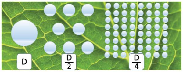
As a consequence, the optimal droplet size distribution is a matter of careful optimization: while a fine spray can take advantage of air turbulence and be beneficial for improving coverage in a dense canopy, medium-coarse spray is preferred to decrease drift risks with product losses in air, water, and soil. Coarse to very coarse sprays need to be used when wind velocity is above the optimal range (1–3 m s−1) and treatments cannot be postponed.
Action Mode and Application Parameters
Spray characteristics have to be adapted to the features of the target and crop and to the pesticide action mode. There are mainly two broad groups of pesticide modes of action: contact pesticides, with a protection efficacy restricted to the areas directly reached by the chemical in a sufficient amount; and systemic pesticides, with a protection efficacy depending on the overall absorption by the plant of a sufficient amount of chemical and its internal translocation to the site of action.
Contact products generally require high deposit densities (75–150 droplets cm−2) for a dense coverage of the target surface, as obtained with closely spaced droplets of finer sprays. On the other hand, for systemic products, coverage of the surface is less important provided that a sufficient dose of pesticide is delivered to, and absorbed by, the plant. Hence, lower deposit densities (20–40 droplets cm−2) are used, associated with coarser sprays.
Application Rate
By combining the droplet size and deposit density chosen for a pesticide treatment, the application rate AR, i.e., the liquid volume per unit of sprayed area, can be computed as:
\( AR = \frac{\text{liquid volume}}{\text{sprayed area}} = (\text{mean drop volume})(\frac{\text{number of drops}}{\text{sprayed area}}) \)
The determination of the sprayed area should take into account that, for soil treatments, the target surface is the field area, whereas for plant treatments, it is the total vegetation surface of the plant. The relationship between the two is usually expressed as leaf area index, LAI, which is the ratio between the leaf surfaces of the target and the surface of the field in which it is growing. At early stages of growth, an LAI of about 1 is usually assumed (as for soil), while with further development LAI increases to 5 or more, depending on the crop. The previous expression can then be rewritten as:
\( AR = \frac{4}{3}\pi (\frac{VMD}{2})^{3} \times n_{d} \times LAI = \frac{\pi}{6} VMD^{3}(\mu m^{3})(10^{-15}L \ \mu m^{3}) \times n_{d}(cm^{-2})(10^{8} cm^{2} ha^{-1}) \times LAI \)
that is,
\[ AR = 10^{-7} \times \frac{\pi}{6} VMD^{3} \times n_{6}\times LAI \]
where AR = application rate (L ha−1)
VMD = volume median diameter of the spray (μm)
nd = the deposit density on the target surface (number of droplets cm−2)
LAI = leaf area index of sprayed plants (decimal; = 1 for soil and early growth stages)
Functional Components of the Sprayer
The sprayer is the machine that carries, meters, atomizes, and applies the spray material to the target. The main functional components of a sprayer are shown in Figure 3.2.10.
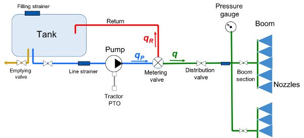
The tank contains the water-pesticide mixture to be applied, with capacities that vary from 10 L for human-carried knapsack models to more than 5 m3 for large self-propelled sprayers. Tanks are made of corrosion-resistant and tough material, commonly polyethylene plastic, suitably shaped for easy filling and cleaning. To keep uniform mixing of the liquid in the tank, suitable agitation is provided by the return of a part of the pumped flow or, more rarely, by a mechanical mixer.
The pump produces the liquid flow in the circuit, working against the resistance generated by the components of the system (valves, filters, nozzles, etc.) and by viscous friction. The higher the resistance that the pump must overcome, the greater the pressure of liquid in the circuit.
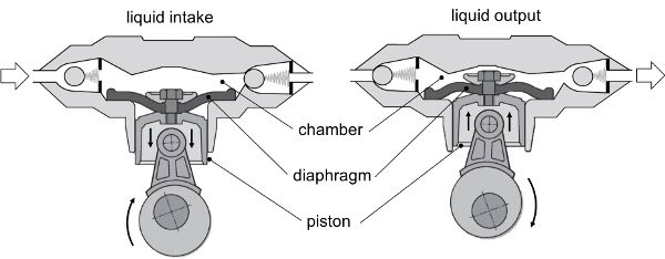
Diaphragm pumps (Figure 3.2.11) are the most common type used in sprayers, because they are lightweight, low cost, and can handle abrasive and corrosive chemicals. The pumping chamber is sealed by a flexible membrane (diaphragm) connected to a moving piston. When the piston moves to increase the chamber volume (Figure 3.2.11, left), liquid enters by suction through the inlet valve. As the piston returns, the diaphragm reduces the chamber volume (Figure 3.2.11, right), propelling the liquid through the outlet valve.
As for any positive displacement pump, diaphragm pumps deliver a constant flow for each revolution of the pump shaft, regardless of changes of pressure (within the working range):
\[ q_{p} = 10^{-3}V_{p}n_{p} \]
where qp = flow rate delivered by the pump (L min−1)
Vp = pump displacement (cm3)
np = rotational speed of the pump shaft (min−1)
In tractor-coupled sprayers, the pump is actuated by the tractor PTO shaft to provide the spraying liquid hydraulic power necessary to operate the circuit. The hydraulic power is:
\[ P_{hyd} = pq_{p}/ 60000 \]
where p = pressure of the circuit (kPa)
qp = flow rate produced by the pump (L min−1)
Some sprayers use centrifugal pumps. In these cases, the flow from the pump will not be positive displacement and will depend upon the pressure the pump has to pump against.
Control valves in the circuit enable the desired functioning of the sprayer, by controlling flow direction and volume in the different sections, and by maintaining a desired liquid pressure that, in turn, defines the spray characteristics and the distributed volume.
Since pressure is a fundamental parameter for spray distribution, a pressure gauge with appropriate accuracy and measurement range (e.g., two times the expected maximum pressure) is always installed in the sprayer circuit.
Nozzles are the core component of the sprayer that atomizes the pesticide-water mixture into droplets, producing a spray with a specific pattern to cover the target. The most common atomizing technology in sprayers is the hydraulic nozzle (Figure 3.2.12), which breaks up the stream of liquid as it emerges by pressure from a tiny orifice into spray droplets.
For a given liquid (i.e., for a given density and surface tension), the operating pressure and the orifice area directly determine the size of the droplets of the produced spray. In particular, by increasing the pressure with a specific nozzle, the size of the droplets decreases. Conversely, for a given pressure the size of the droplets increases with the area of the nozzle orifice.
Flow Rate Metering by Pressure Control
The discharge flow rate through a nozzle with a given orifice size can be metered by setting the liquid pressure in the circuit before the nozzle. The Bernoulli equation, which describes the conservation of energy in a flowing liquid, can be applied to the liquid flow at two points of the nozzle body: one in the nozzle chamber before entering the nozzle orifice (point 1 in Figure 3.2.12) and the other at the outlet of the orifice (point 2 in Figure 3.2.12). Neglecting the energy losses due to viscous friction, the Bernoulli equation gives:
\( P_{1} + \frac{1}{2}\rho \nu_{1}^{2} + \rho gz_{1} = p_{2}+ \frac{1}{2} \rho \nu_{2}^{2} + \rho gz_{2} \)
where p1 = absolute pressure of the liquid in the circuit
p2 = atmospheric pressure
ρ = density of the liquid
v1 and v2 = mean velocities of the liquid before entering the orifice and just after it
g = acceleration due to gravity
z1 and z2 = vertical positions of the two considered points
From flow continuity, it is also obvious that:
qn= A1⋅v1 = A2⋅v2
where qn = flow rate through the nozzle
A1 and A2 = area of sections of the nozzle chamber and orifice, respectively
Due to the tiny diameter of the orifice, the fluid velocity v2 in the orifice is much larger than that in the chamber v1, which can be neglected in the equation. Moreover, due to the small distance between the two points, we can consider z1 ≅ z2. The Bernoulli equation for the nozzle then simplifies as:
\( p \simeq \frac{1}{2} \rho (\frac{q_{n}}{A})^{2} \)
that can be rearranged, leading to the nozzle equation:
\[ q_{n} = 1.0 c_{d}A_{o} \sqrt{\frac{2p}{\rho}} \]
where qn = flow rate discharged by the nozzle (L min−1)
1.9 = a constant resulting from units adjustment
cd = discharge coefficient that accounts for the losses due to viscous friction through the orifice = <1 (decimal) (typically proportional to v22)
Ao = area of the nozzle orifice (mm2)
p = operating pressure of the circuit (kPa), i.e., p = p2 – p1 the differential pressure to the atmosphere
In practical applications, Equation 3.2.16 is used in the form:
\[ q_{n} = k_{n} \sqrt{p} \]
where kn is a nozzle-specific efflux coefficient that incorporates its construction characteristics and viscous losses. The value of kn (commonly in the range of 0.03 to 0.2 L min−1 kPa−1/2) can be derived from flow-pressure tables provided by the nozzle manufacturer.
Equation 3.2.17 shows that the discharged volume rate of pesticide-water mixture can be varied by adjusting the circuit pressure p. Increasing the pressure will increase the flow rate and decrease the spray droplet size simultaneously. However, there is usually a limited working range of pressure (depending on nozzle type, this can be from 150 kPa up to 800 kPa, rarely above) because outside that range, the spray droplets will be either too large or too small. In this working range of pressure, the flow rate increases proportionally to the square root of pressure; if larger changes in discharge rate are needed, a nozzle with a different orifice area (i.e., different kn) has to be selected.
Sprayer Application Rate Metering
For a required application rate AR (corresponding to a defined dose of pesticide), the sprayer volume rate, q, to be discharged in the field has to be set to a value computed by applying Equation 3.2.12, which includes the operating speed and width of the machine. By dividing the total outflow rate q by the number of nozzles equipping the sprayer, the nozzle flow rate qn is obtained.
Once an appropriate nozzle is chosen (i.e., a nozzle able to deliver qn within the usual working range of pressures), the circuit pressure has to be fine tuned, by means of the control valve, until the liquid pressure value (read on the pressure gauge) is the one obtained by solving Equation 3.2.17 for p and using the kn value from the nozzle manufacturer, i.e.:
\[ p = (\frac{q_{n}}{k_{n}})^{2} \] Figrue
This relationship is also used in sprayer electronic controllers to achieve a constant application rate as the sprayer speed varies, or to adjust the application rate for different areas in the fields.
Applications
The concepts and calculations discussed above are widely used to design crop production equipment, and also for the adjustment and management of equipment to suit local conditions on individual farms.
Tillage Equipment
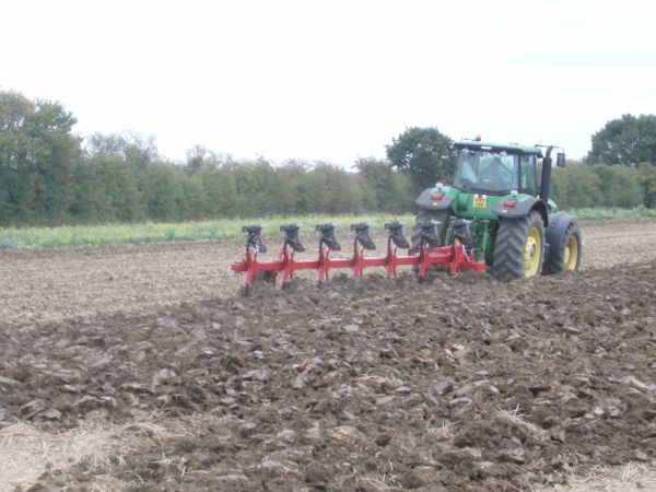
Plows are used for deep tillage operations and are unique in soil movement as they invert soil to be almost upside down, as shown in Figure 3.2.13. Disc plows cultivate the soil in shallow layers aiming at weed elimination, loosening the soil and uprooting crop plants remaining after harvest.
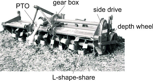
In contrast, PTO-driven implements (such as shown in Figure 3.2.14) cultivate the soil more intensively, breaking it into smaller pieces. The intensity is controlled by the axle rotation speed and the tractor speed resulting in a bite length as pointed out by Equation 3.2.4. Powered implements use the engine power of the tractor more efficiently because slip of wheels due to non-optimal track conditions in the fields are avoided. They are smaller than primary tillage machines in length and weight and are therefore appropriate for combining with other tillage tools (e.g., rollers) or seed drills.
Some other implements used on farms for primary and secondary tillage are illustrated in Figure 3.2.15.
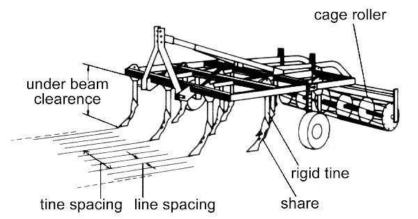
(a)
(b)
Figure \(\PageIndex{15}\): (a) Tine cultivator with tines line spacing and tine spacing; (b) disc cultivator in A-type formation to compensate lateral forces.
Planting Equipment
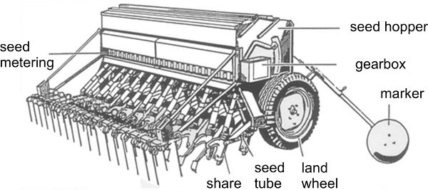
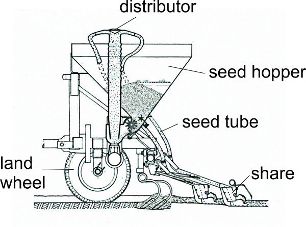
The most common technique in sowing seeds is drilling with metering by wheels for each row as shown in Figure 3.2.16. Each row needs a metering wheel and a share. The hopper supplies all rows and extends over the entire working width. The metering wheels grasp seeds from the hopper bottom and transport them over a bottom flap to drop them via the seed tubes into the share and from there into the soil. As a result, the seeds are not distributed in the row with constant distances but are placed randomly. The function of the marker (Figure 3.2.16a) is to guide the tractor in the subsequent path.
Centralized hoppers can increase capacity of seeding machines. The centralized hopper has only one metering wheel, under the conical hopper bottom. An air stream conveys the grain via a distributor to the shares using flexible pipes.
(a)
(b)
Figure \(\PageIndex{16}\): (a) Regular seed drill; (b) pneumatic seed drill.
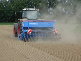
Seeds can be sown in well prepared soil (after secondary tillage), which is the regular case (Figure 3.2.17), or under other soil conditions when minimum tillage or no till is applied. Minimum tillage cultivates the soil without deep intervention (e.g., plowing) and no tillage means seeding without any tillage manipulation of the soil. A typical part of the seeding machine is the hopper for fertilizer (between tractor and seeder; Figure 3.2.17b). This combination offers fertilization and seeding in the same pass.
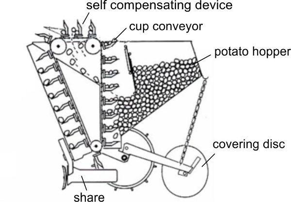
Machines that plant potatoes, transplant seedlings, and so on, have mechanisms that are quite varied, depending upon what is to be planted into the soil. One example for potatoes is displayed in Figure 3.2.18a. A chain with catch cups passes through a pile of potatoes in the hopper and picks up potatoes. If there is more than one potato on a cup, the excess potatoes fall off in the horizontal section. The potatoes are then transported down and placed at a constant separation distance in the open furrow.
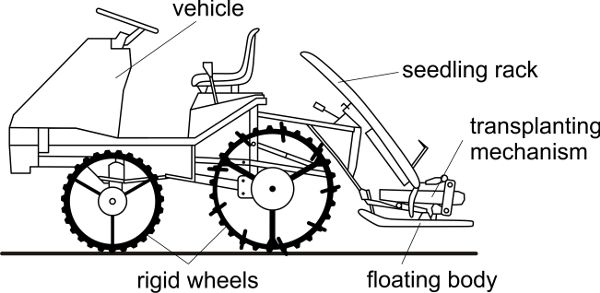
A rice transplanter is displayed in Figure 3.2.18b. The seedlings are kept in trays gliding down to the transplanting mechanism. A crank arm for each row will pick out a single seedling and place it in the soil.
(a)
(b)
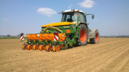
Figure \(\PageIndex{17}\): (a) Tractor-mounted seed drill working in a well prepared soil with small wheels for recompaction of the cover soil after embedding the seeds (wheat); (b) precision seeder sowing maize (corn) in well prepared soil with larger recompaction wheels.
Fertilizer Distribution Equipment
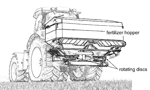
The most common fertilization equipment is the centrifugal spreader (Figure 3.2.19). This machine is often powered by a tractor through the PTO shaft and often mounted on the tractor’s three point-hitch. Large units (hopper capacity above 1500 kg) can have their own wheels and be pulled by a tractor, or be mounted on trucks. The fertilizer granules flow by gravity, with aid of an agitator, from two outlets on the hopper bottom. The outlets area is adjustable through a sliding gate, which meters the mass outflow Q (kg min−1) to control the rate of fertilizer application to the field.
(a)
(b)
Figure \(\PageIndex{18}\): (a) Potato transplanter with device to complete the filling of cups; (b) rice transplanter with device moving the seedlings from the tray in the soil.
Under the outlets, the metered fertilizer drops on rotating discs (30 to 50 cm in diameter) that impart a centrifugal force on the fertilizer granules, thus distributing them at distances that can reach 50 m. Nevertheless, the working width of centrifugal spreaders is typically 18–24 m and rarely higher than 30 m. Centrifugal spreaders do not uniformly deposit the fertilizer across the working width, but rather with a triangular pattern that requires a partial overlap between two adjacent passes to obtain a uniform transversal distribution within the field. Field speeds typically range from 8 to 12 km h−1, but smooth ground conditions can enable applications faster than 15 km h−1.
Liquid Fertilizer Distributors
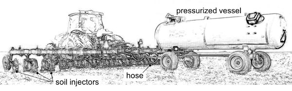
Use of liquid mineral fertilizers is rather limited in Europe, except in vegetable crops where the nutrient solution is distributed by a sprayer (see next section) or, much more frequently, in association with irrigation through micro-irrigation systems (fertigation). On the other hand, in North America, fertilization with liquid anhydrous ammonia is very common due to its high nitrogen content (82%) and low cost. Non-refrigerated anhydrous ammonia is applied from high pressure vessels, and it has to be handled with care to prevent hazardous situations. Equipment for application (Figure 3.2.20) includes injectors mounted on soil-cutting knives spaced 20–50 cm apart that reach a depth of 15–25 cm in the soil. When delivered in the soil, the ammonia turns from liquid into gas that reacts with water and rapidly converts to ammonium made available to plant roots. This molecule strongly adheres to mineral and organic matter particles in the soil, helping to prevent gaseous or leaching losses.
Slurry Tankers
A slurry tanker (Figure 3.2.21) is commonly used for distributing organic fertilizer in areas with livestock. The tanker is a trailed, massive piece of equipment mounted on a single or double axle frame (or three axles for tank capacity above 20 m3) equipped with wide wheels (up to 800 mm) to reduce soil compaction. In vacuum tankers, the stainless steel tank is pressurized at 150–250 kPa for spreading by compressed air, which is pumped in. During tank filling, the pump produces a negative pressure difference (vacuum) with the atmospheric pressure, enabling the slurry to be sucked into the tank by a flexible pipe. Slurry flow can also be obtained with direct slurry pumping by a multiple-lobe pump.
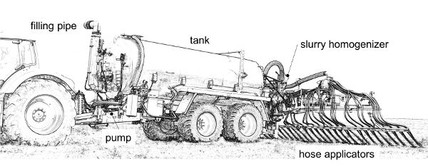
Traditional distribution from a slurry tanker involves a deflector or splash plate mounted on the back of the tank. The slurry impacts the plate and thus is spread over an umbrella pattern covering a width of 4–8 m. Splash plates have been banned by legislation in some countries due to odor emission and nutrient losses (e.g., by ammonia volatilization), so they have been replaced by soil applicators. Soil applicators have multiple hoses mounted on a horizontal boom ending with trailed openings, spaced about 20–30 cm apart, that deposit the slurry flowing through the hose directly on the soil. The soil applicator can also be an injector, made of a tine or a vertical disc tool, that makes a groove in the ground where the slurry is injected at depths ranging from 5 cm (for meadows) to 15–20 cm (tilled soil).
To obtain a uniform distribution of slurry flow among the multiple hose lines, soil applicators require the adoption of a homogenizer. This is a hydraulically-driven shredding unit that processes the slurry with rotating blades to cut fibers and clogs to ensure the regular and even feeding of all the hoses connected to the injectors.
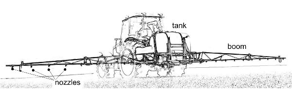
Sprayers
In addition to the common functional parts of sprayers (tank, pump, valves, boom, nozzles), sprayers are manufactured in a wide variety of types for specific crops, various application techniques, environmental regulations, purchase costs, etc. CIGR (1999) provides information about various types of sprayers.
Boom sprayers (Figure 3.2.22) are the main type used for protection treatments on field crops (e.g., cereals, vegetables, and leguminous crops). They are named for the wide horizontal boom where nozzles are mounted. Booms often range from 8 to 36 m (and sometimes more) in width, with a height from the soil adjustable from 30 cm to more than 150 cm to ensure a good spray pattern at the level of the target. The boom is generally self-leveling to reduce travel undulation and provide more uniform spray application.
Nozzles are mounted on the booms with a typical spacing of 50 cm, although the spacing may range from 20–150 cm depending upon the specific application and the type of nozzle. The most used nozzle on boom sprayers is the fan type that can produce a wide spectrum of droplet size, from medium-fine to coarse spray, at low pressure (150–500 kPa), meeting most field crop spraying requirements.
A boom sprayer is commonly mounted on a tractor by the three point-hitch, or in the case of sprayers with large capacity tanks (above 1 m3), may be a trailed unit pulled by a tractor or self-propelled. Operating speed can vary, largely with field conditions and type of treatment, but during accurate protection treatments a speed range of 7–10 km h−1 is typical.
Examples
Example \(\PageIndex{1}\)
Example 1: Work rate and timeliness of row-crop planting
Problem:
A farmer has a six-row planter for planting maize with a row spacing of 75 cm. The farmer wants to know the field capacity of the planter and whether it can successfully plant 130 ha within five working days. If not, what size planter could do this task?
Assumptions:
- • Forward speed, s, = 9 km h−1. This is a typical value that depends on the seedbed (firmness, levelness, residue, etc.) and the characteristics of the equipment
- • Field efficiency, ef, = 0.65. This typical value allows for non-planting times, such as filling the planter with seeds and turning at the end of rows.
- • Five working days. This is given, but is very dependent upon the weather.
- • Eight hours per day of effective field time. This is the time that the planter is available for field work and does not include time for machine preparation, transfer to fields, operator breaks, and other non-planting activities.
Solution
The first step is to calculate the field capacity, Ca, using Equation 3.2.2:
\( C_{a} = 0.1 e_{f}\ w \ s \) (Equation \(\PageIndex{2}\))
We are given ef and s. The planter’s operating width, w, can be calculated as:
\( \text{number of rows} \times \text{width per row} = 6 \text{ rows} \times 75 \text{ cm row}^{-1} \times (m/ 100 \ cm) = 4.5 m \)
Substituting the values into Equation 3.2.2:
\( C_{a} = 0.1 \times 0.65 \times 4.5m \times 9 \text{ km h}^{-1} = 2.63 \text{ ha h}^{-1} \)
Therefore, the planter is capable of planting 2.63 ha every hour. If the planter is used to plant on five days for eight hours on each day, the area planted in that time is:
\( A = (2.63 \text{ ha h}^{-1} \times (5 \text{ days} \times (8 \text{ h day}^{-1}) = 105.2 \text{ ha} \)
That is less than the required 130 ha. Perhaps the farm staff will have to work more hours, but one option for the farmer would be to get a larger planter, which may require a larger tractor. The following calculations help the farm manager select equipment and manage its use.
The field capacity of the new planter needs to be:
\( C_{a} \geq (130 \text{ ha}) / (40 \ h) = 3.25 \text{ ha h}^{-1} \)
Then, by rearranging Equation 3.2.2 the minimum operating width can be computed:
\( w \geq (3.25 \text{ ha h}^{-1}) (10)/ ( 0.65 \times 9 \text{ km h}^{-1}) = 5.56 \text{ m} \)
This width corresponds to a number of rows:
\( Nr \geq (5.56 \text{ m}) / ( 0.55 \text{ m row}^{-1}) = 7.41 \text{ rows} \)
Therefore, the farmer should get an 8-row planter (i.e., the next market size ≥ 7.41) to accomplish the planting of 130 ha within 40 hours of work.
Example \(\PageIndex{2}\)
Example 2: Draft force while plowing
Problem:
When designing the frame and hitch of a plow, an engineer needs to know the draft force to ensure that the frame and hitch have enough strength. The draft force also affects tractor selection, since the draft force and speed determine the required pulling power. Determine the draft force needed to pull the plow at a speed of 7 km h−1 given the following information about the plow:
- • 4-share plow
- • 1 gauge wheel
- • 5000 N weight on gauge wheel
- • 0.15 gauge wheel rolling resistance factor
- • 40 cm furrow width
- • 30 cm furrow depth
- • 5 N cm−2 static factor
- • 0.21 N s2 m−2 cm−2 dynamic factor
Solution
Calculate the draft force using Equation 3.2.3:
\( F_{z} =nF_{v}\rho _{r} + ikw_{f}d+i\epsilon w_{f}dv^{2} \) (Equation \(\PageIndex{3}\))
where Fz = draft force (N)
n = number of gauge wheels = 1
Fv = vertical force = 5000 N
ρR = rolling resistance = 0.15
i = number of moldboards or shares = 4
k = static factor = 5 N cm−2
wf = width of furrow = 40 cm
d = depth of furrow = 30 cm
ε = dynamic factor = 0.21 N s2 m−2 cm−2
v = traveling speed = 7 km h−1
Draft force \(F_{z}=1 \times 5000 \times 0.15 + 4 \times 5 \times 40 \times 30 + 4 \times 0.21 \times 40 \times 30 \times 7 = 31,806 \text{ N}\)
Example \(\PageIndex{3}\)
Example 3: Length of a rotovator (rotary tiller) bite
Problem:
Determine the bite taken by each blade on the rotary tiller with these characteristics:
- • rotary tiller turning at 240 revolutions per minute
- • travelling at 5 km h−1
- • 4 blades on each tool assembly
Solution
Use Equation 3.2.4:
\( B = \frac{\nu \ 10,000}{n \ z \ 60} \) (Equation \(\PageIndex{4}\))
where B = bite length
v = travel speed = 5 km h−1
n = rotary speed = 240 min−1
z = number of blades per tool assembly = 4
Bite length, \( B= 5 \times 1000 / (240 \times 4 \times 60) = 8.68 \text{ cm} \)
Each blade takes an 8.68 cm bite. The size of this bite will affect the properties of the tilled soil.
Example \(\PageIndex{4}\)
Example 4: Nitrogen fertilization with a centrifugal spreader
Problem:
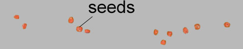
A test was conducted to determine if nitrogen fertilizer was being applied uniformly at the target application rate. The situation is described by the following:
- • centrifugal spreader with working width of 18 m
- • travel speed of 9 km h−1
- • desired nitrogen dose of 70 kgN ha−1
- • calcium ammonium nitrate is 27% nitrogen
- • spreader hopper holds 1000 kg of calcium ammonium nitrate
- • spreader tested with 50 cm by 50 cm trays collecting applied fertilizer
- • figure below shows the amount of fertilizer that was collected in each tray while testing the spreader
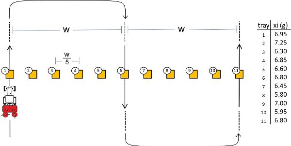
Analyze the collected data to determine the following:
- (a) spreader flow rate (kg/min) of calcium ammonium nitrate to achieve desired nitrogen dose
- (b) time between fillings of the hopper
- (c) average application rate and coefficient of variation from the test
Solution
- (a) By applying Equation 3.2.10, the amount of calcium ammonium nitrate needed to achieve 70 kgN ha−1 is:
- \( D = c_{AC} AR \) (Equation \(\PageIndex{10}\))
where D = dose of application = 70 kgAC ha−1
cAC = content of active compound in the raw material = 0.27 kgN kg−1
AR = application rate
Rearranging and using the given information,
- \( AR= (70 \text{ kg}_{N}\text{ha}^{-1})/ (0.27 \text{ kg}_{N}\text{kg}^{-1}) = 259.3\text{ kg}\text{ ha}^{-1} \)
- This corresponds to a flow rate of the fertilizer (Equation 3.2.11):
- \( Q = AR \ w \ s / 600 \) (Equation \(\PageIndex{11}\))
- \( Q = (259.3 \text{ kg ha}^{-1}) \times 18 \text{ m} \times 9 \text{ km min}^{-1} / 600 (\text{min h}^{-1}) (\text{ m km ha}^{-1}) = 70 \text{ kg min}^{-1} \)
- Therefore, the flow out of the spreader must be adjusted to 70 kg min−1.
- (b) The time between fillings is the time it takes to spread all the fertilizer from the spreader:
- \( t = 1000 \text{ kg} / (70 \text{ kg min}^{-1}) = 14.3 \text{ mins} \)
- The hopper must be refilled every 14.3 minutes.
- (c) The average amount applied is found by summing the amounts of fertilizer in the trays and dividing by the number of trays:
- \( \bar{x} = (6.95+7.25+6.30+ …+6.80)/11=6.62\text{ g} \)
- The mean application rate can be found by dividing that amount by the surface area of a tray:
- \( \text{Mean AR} = \bar{x}/(\text{area of tray}) \)
- \( = (6.62 \text{ g}) \times (\text{kg}/1000 \text{ g}) / [(0.5 \text{ m}) \times (0.5 \text{ m}) \times (\text{ ha} /10000 \text{ m}^{2})]=264.8 \text{ kg ha}^{-1} \)
- That is close to the desired rate, but represents an error of:
- \( [(264.8 - 259.3)/259.3] \times 100\text{%}=2.1 \text{% error} \)
The uniformity of distribution is quantified by the coefficient of variation (CV) of the collected material as shown by Equation 3.2.6:
- \( CV = \frac{\sqrt{\frac{\sum{(x_{i}-\bar{x})^{2}}}{N-1}}}{\bar{x}} 100\text{%} \) (Equation \(\PageIndex{6}\))
where CV = coefficient of variation (%)
N = number of measured samples
xi = amount of fertilizer collected in each tray (g)
\(\bar{x} \)= mean amount (g)
That is, by using the appropriate values given in the fertilizer test figure:
- \( CV = \sqrt{\frac{(6.95-6.62)^{2} + (7.25-6.62)^{2} + (6.30 - 6.62)^{2}+…+(6.80-6.62)^{2}}{11-1}}\times \frac{100 \text{%}}{6.62} = 6.2 \text{%} \)
- Since a coefficient of variation under 10% is considered good, the field test shows that the spreader is performing satisfactorily.
Example \(\PageIndex{5}\)
Example 5: Sprayer pressure setting
Problem:
A fungicide treatment has to be sprayed to a crop at an application rate, AR = 250 L ha−1. For this kind of treatment the farmer mounts nozzles that deliver a flow qn = 1.95 L min−1 at a circuit pressure of 400 kPa. (This information is provided by the nozzle manufacturer.) Determine the proper pressure to be set in the sprayer circuit in order to distribute the fungicide at the desired application rate.
Assumptions:
- • boom width, w, = 24 m with a typical nozzle spacing, d, = 50 cm
- • forward speed, s, = 8 km h−1, usual for fungicide treatments (depends on wind conditions)
Solution
The first step is to calculate the volume rate q (L min−1) required to distribute the application rate by applying Equation 3.2.12:
\( q = AR \ w \ s / 600 \) (Equation \(\PageIndex{12}\))
Substituting the given values into the equation:
\( q = 250 \text{ L ha}^{-1} \times 24 \text{ m} \times 8 \text{ km h}^{-1} / 600 = 80 \text{ L min}^{-1} \)
The number of nozzles equipping the boom is:
\( (24 \text{ m}) / (0.50 \text{ m nozzle}^{-1}) = 48 \text{ nozzles} \)
The required flow rate per nozzle qn is:
\( q_{n}=(80 \text{ L min}^{-1}) / (48 \text{ nozzles}) = 1.67 \text{ L min}^{-1} \)
In order to choose the pressure setting to obtain the desired flow of 1.67 L min−1 we need to calculate, for these nozzles, the discharge coefficient kn of Equation 3.2.17:
\( q_{n}= k_{n} \sqrt{p} \) (Equation \(\PageIndex{17}\))
By substituting the values provided by the nozzle manufacturer (qn = 1.95 L min−1, p = 400 kPa) we find:
\( k_{n} = \frac{1.95 \text{ L min}^{-1}}{\sqrt{400 \text{ kPa}}} = 0.0975 \)
Then, by Equation 3.2.18 we compute the set value of the sprayer circuit pressure:
\( p = (\frac{q_{n}}{k_{n}})^{2} \) (Equation \(\PageIndex{18}\))
\( p = (\frac{1.67}{0.0975})^{2} = 293 \)
Thus, the metering valve has to be adjusted until the circuit pressure reads 293 kPa (2.93 bar) on the pressure gauge.
Image Credits
Figure 1. Oberti, R. (CC By 4.0). (2020). Typical operations involved in growing field crops.
Figure 2. Oberti, R. (CC By 4.0). (2020). The field capacity of a machine.
Figure 3. Schulze Lammers, P. (CC By 4.0). (2020). (a) Moldboard plow body. (b) Chisel tine of a cultivator. (c) Disc plough.
Figure 4. Schulze Lammers, P. (CC By 4.0). (2020). Seed distribution (a) drilled seed, (b) band seed, (c) broadcasted seed, (d) precision seed.
Figure 5. Schulze Lammers, P. (CC By 4.0). (2020). Studded seed wheel for metering seeds, with bottom flap for adjustment to seed size.
Figure 6. Schulze Lammers, P. (CC By 4.0). (2020). (a) Seed deposition, drilled. (b) Frequency of seed distances, drilled.
Figure 7. Schulze Lammers, P. (CC By 4.0). (2020). Fluted pipe with plate for distribution of seeds along the circumference into the seed tubes, and cell wheel in detail.
Figure 8. Schulze Lammers, P. (CC By 4.0). (2020). Precision seeder singling seed grains for seed placement with definite spacing, (a) mechanical singling by cell wheel. (b) pneumatic singling device with cell wheel.
Figure 9. Oberti, R. (CC By 4.0). (2020). Reducing droplet size.
Figure 10. Oberti, R. (CC By 4.0). (2020). Schematic diagram of a sprayer.
Figure 11. Mancastroppa, S. (CC By 4.0). (2020). Diaphragm pump.
Figure 12. Oberti, R. (CC By 4.0). (2020). Hydraulic nozzle operation.
Figure 13. Schulze Lammers, P. (CC By 4.0). (2020). Tractor mounted moldboard plow working in the field.
Figure 14. Schulze Lammers, P. (CC By 4.0). (2020). Rotary tiller as an example of a PTO-driven tillage implement.
Figure 15. Schulze Lammers, P. (CC By 4.0). (2020). (a) Tine cultivator with tine line spacing and tine spacing. (b) Disc cultivator in A-type formation to compensate lateral forces.
Figure 16. Schulze Lammers, P. (CC By 4.0). (2020). (a) Regular seed drill. (b) Pneumatic seed drill.
Figure 17. Schulze Lammers, P. (CC By 4.0). (2020). (a) Tractor mounted seed drill working in a well prepared with small wheels for recompaction of cover soil after embedding the seeds (wheat). (b) Precision seeder sowing maize in well prepared soil with larger recompaction wheels.
Figure 18. Schulze Lammers, P. (CC By 4.0). (2020). (a) Potato transplanter with device to complete the filling of cup grippers. (b) Rice transplanter with device moving seedlings from the tray in the soil.
Figure 19. Mancastroppa, S. (CC By 4.0). (2020). Centrifugal fertilizer spreader.
Figure 20. Mancastroppa, S. (CC By 4.0). (2020). Equipment for anhydrous ammonia.
Figure 21. Mancastroppa, S. (CC By 4.0). (2020). Slurry tanker.
Figure 22. Mancastroppa, S. (CC By 4.0). (2020). Boom sprayer.
Example 4. Oberti, R. (CC By 4.0). (2020).
References
ASABE Standards. (2017). ANSI/ASABE S572.1: Spray nozzle classification by droplet spectra. St. Joseph, MI: ASABE.
CIGR. (1999). Plant production engineering. In B. A. Stout & B. Cheze (eds). CIGR handbook of agricultural engineering (vol. 3). St. Joseph, Michigan: ASAE.
Gorjachkin, W. P. (1968). Sobranie socinenij (vol. 2). Moscow: Kolow Press.
Heege, H. J. (1993). Seeding methods performance for cereals, rape, and beans. Trans. ASAE, 36(3): 653-661. https://doi.org/10.13031/2013.28382.
Müeller, J., Rodriguez, G., & Koeller, K. (1994). Optoelectronic measurement system for evaluation of seed spacing. AgEng ’94 Milano Report N. 94-D-053.
Schilling, E. (1962). Landmaschinen (2nd ed., p. 288).