3.3: Grain Harvest and Handling

Tim Stombaugh

Biosystems and Agricultural Engineering

University of Kentucky

Lexington, Kentucky, USA

Key Terms

Performance	Efficiency	Dissociation
Productivity	Functional processes	Separation
Quality	Engagement	Transport

Variables

Note about units: In this list of variables, dimensions of variables are given. In the text, variable definitions include dimensions as well as example SI units for illustration.

• ε = strain
• η_v = volumetric efficiency of the conveyor
• θ = angular position of rotating support, or connecting, arms
• ρ_air = density of the air in mass per volume
• ρ_grain = density of the grain
• σ = stress in units of force per unit area
• σ_b = bending stress in the connective tissue in force per unit area
• σ_t = tensile stress in the connective tissue in force per unit area
• σ_y = yield stress in force per unit area
• ω = rotational speed
• a = acceleration of the particle in the direction of the resultant force in length per time squared
• A = cross-sectional area of connective tissue or structural member
• A_part = characteristic area of the particle
• C_a = effective field capacity in area per unit time
• C_d = drag coefficient of the particle
• C_m = material capacity in weight or volume per unit time
• d = diameter of shaft
• D = outside diameter of the flighting
• E = modulus of elasticity in force per unit area
• E_f = field efficiency
• E_h = harvest efficiency
• F = force in the member
• F_d = drag force
• F_g = gravitational force
• F_r = resultant force on the particle
• F_t = tensile force acting on connective tissue
• g = gravitational constant in length per unit time squared
• h = height that the material is lifted
• I = moment of inertia of the connective tissue cross section in mass x length squared
• L = length of a structural member
• L_h = total harvest loss
• L_s = separation loss
• L_sh = shatter losses
• L_th = threshing loss
• m = mass of the particle
• M = bending moment in force x distance
• n = number of paddles that are discharged per unit time
• Q_a = actual volumetric flowrate of grain in volume per unit time
• Q_t = theoretical flowrate in volume per unit time
• P = pitch length of the flighting
• P_g = power required to overcome gravity in (force x distance) per unit time
• r = length of rotating support, or connecting, arms
• R_w = total weight that the cart wheels and axles must support
• s = field speed in distance per unit time
• T_a = actual completion time
• T_t = theoretical completion time
• v = velocity in length per time
• v_f = forward speed
• v_part = velocity of the particle relative to the air
• v_h = horizontal component of tangential velocity
• v_t = tangential velocity
• v_v = vertical component of tangential velocity
• V = volume of material carried by a single paddle
• w = machine width
• x_g = grain center of gravity
• y = perpendicular distance to neutral axis
• y_a = actual harvested, or recovered, yield of grain in weight or volume per unit area
• y_p = potential yield of grain in the field in weight or volume per unit area
• y_ph = pre-harvest yield loss in weight or volume per unit area
• y_t = total yield that the plants actually produced in weight or volume per unit area

Introduction

One unique skill that biosystems engineers must develop is the ability to understand how mechanical systems interact with biological systems. This interaction is very prevalent in the design of machinery and systems for harvesting grains such as corn (maize, Zea mays), soybean (Glycine max), wheat (Triticum), or canola (Brassica napus). The machines must traverse through a field on a biologically active soil to engage the plants growing in that field. The variability in plant and soil properties (e.g., maturity, moisture content, and structural integrity) within a field can be extensive. This variability presents a challenge to design engineers to conceive machines that can accommodate this variability and provide the machine operator with the flexibility needed to properly engage the plants. The goal of this chapter is to lay the engineering foundation needed to design machinery systems for harvesting grain crops.

Outcomes

After reading this chapter, you should be able to:

• • Identify the basic functional processes needed to harvest grain
• • Describe the basic engineering principles governing grain harvest machinery design
• • Quantify machine performance and design basic machine components using basic engineering principles

Concepts

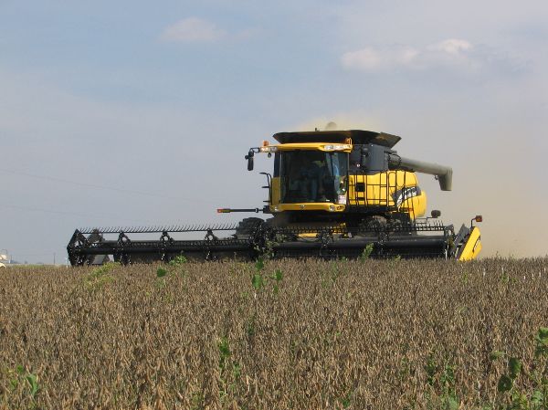
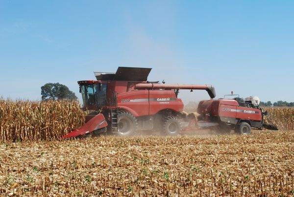
One key to becoming a great engineer is the ability to identify and understand the core problem to be solved. Too often, engineers focus on improving current solutions to problems rather than looking for better solutions. In the case of grain harvest, the engineer might be tempted to focus on ways to improve the grain combine (Figure 3.3.1), which is the machine most commonly used to harvest grain. The most unique and creative engineering solutions will often come only when the engineer focuses on identifying the fundamental problem to be solved.

With grain harvest, the core challenge is to recover a certain fraction or fractions of the plants in a grain crop that is grown in large fields. The fraction that is to be retrieved may vary by plant and by situation. In corn (maize, Zea mays) harvest, for example, the most commonly harvested plant fraction is the kernel, which is used in a variety of products including food, sugar, and biofuel production. For fresh market sweet corn harvest, the whole ear is recovered with the husks intact. In some animal production systems, the whole ear without husks is recovered for animal feed; in other animal production systems, the entire plant is harvested and ensiled for feed. In these examples, the maturity and moisture content of the plant material may be drastically different if the corn is being recovered for sugar production, animal feed, or human consumption. A further challenge may exist where multiple plant fractions are harvested for different purposes. In industrial hemp (cannabis) production, for example, the seeds of the plant might be recovered for oil or food production, and the plant stems might be recovered separately for fiber production. The plurality of production streams will not be independent of each other and must be considered in the design of the mechanization solution. This chapter focuses on systems where only the grain is recovered.

Figure \(\PageIndex{1}\): Typical grain combine with grain table header harvesting a soybean crop.

Performance

The performance of a grain harvesting machine or system can be measured using three general metrics: productivity, quality, and efficiency.

Productivity

The productivity of a harvesting machine or operation is a measure of how much useful work is accomplished. As described in ASABE Standard EP496.3 (2015a), it can be quantified using two primary metrics. First, it can be measured on an area basis indicating how much of the area of a field was covered per unit time. This metric is expressed as the effective field capacity (C_a) and can be calculated as:

\[ C_{a}=swE_{f} \]

where C_a = effective field capacity in area per unit time (m² h⁻¹)

s = field speed in distance per unit time (m h⁻¹)

w = machine width (m)

E_f = field efficiency (decimal)

Second, productivity can be measured on a material basis indicating how much of the grain is recovered per unit time. Material capacity (C_m) is related to the area capacity by:

\[ C_{m}=C_{a}y \]

where C_m = material capacity in weight or volume per unit time (m³ h⁻¹)

y_a = recovered (harvested) crop yield in weight or volume per unit area (m³ m⁻²)

Table \(\PageIndex{1}\): Bushel weight of common grain crops at standardized moisture content.

Commodity	Moisture Content (%)	Weight (lb/bushel)	Weight (kg/bushel)
Corn (Zea mays)	15.5	56	25.40
Soybean (Glycine max)	13	60	27.22
Sunflower (Helianthus annuus)	10	100	45.36
Wheat (Triticum aestivum)	13.5	60	27.22

Material capacity can be reported on either a volume or mass basis with appropriate density conversion. In international trade, grain quantity is typically reported in metric tons. In U.S. grain production, grain quantity is commonly measured using units of bushels. While a bushel is technically a volume measurement equaling 35.239 L, in grain production it is a unit that reflects a standardized weight of grain at a particular moisture content specified for that grain. The standardized weights of a grain bushel for some common crops are listed in Table 3.3.1.

Quality

The second measure of performance of a mechanized grain harvest system is product quality. Ideally, the product (grain) that is recovered is free from any foreign matter and damage, but this is rarely the case. Small pieces of plant material and other foreign matter are often captured with the grain. The machinery can also cause physical damage to the grains as they pass through the different mechanisms. Machine design, as well as crop and operating conditions, can have an effect on foreign matter and damage, which are often referred to collectively as dockage. The term dockage is used because producers generally incur a financial penalty (docked some amount) from the market value of the grain by the buyer if the grain is damaged, contains excessive foreign matter, or is not at the proper moisture content.

Efficiency

The third measure of performance, efficiency, can be quantified in two ways. The first is a time-based field efficiency (E_f) that relates the actual time required to complete a field operation to the theoretical completion time had there been no delays, such as turning around at the ends of the field, machine repair, and operator breaks. Field efficiency is calculated as:

\[ E_{f} = \frac{T_{t}}{T_{a}} \]

where T_t = theoretical completion time

T_a = actual completion time

Efficiency can also be measured based on the completeness of the harvest operation. This harvest efficiency (E_h) is a measure of the amount of desirable product that is actually recovered relative to the amount of product that was originally available to the harvesting machine. It is calculated as:

\[ E_{h} = \frac{y_{a}}{y_{p}} \]

where y_a = actual yield of grain recovered measured in weight per unit area (kg m⁻²)

y_p = potential yield of grain in the field measured in weight per unit area (kg m⁻²)

The antithesis of harvest efficiency is harvest loss (L_h), which is the amount of grain lost by the harvesting machine per unit area expressed as a percentage of the potential yield. It can be calculated as:

\[ L_{h} = 1-E_{h} \]

When focusing on the harvesting operation, the potential yield of the crop is considered to be the harvestable grain that is still attached to the plants. Potential yield does not consider the grains that have fallen from the plants before the machine engages them. If harvest is delayed after the optimum time, potential yield will often decrease due to natural forces causing seeds to fall from the plants. This pre-harvest yield loss (y_ph) is the amount of grain that is lost before harvest expressed on a per area basis. It is the difference between the total yield that the plants actually produced (y_t) and the potential harvestable yield:

\[ y_{ph} = y_{t}-y_{p} \]

There are often strong interrelationships between productivity, grain quality, and efficiency of grain harvest. For example, an increase in productivity could be realized by an increase in speed or field efficiency; however, grain quality and harvest efficiency may be compromised. Finding the fiscally optimum operation point is a challenge to be addressed by both the design engineer and the machine operator. The engineer must understand the needs of the operator and incorporate the appropriate flexibility of control into the design of the machine.

Functional Processes

When considering the design of any mechanization system, the engineer should first carefully consider the potential processes that will have to be undertaken to complete the task. Srivastava et al. (2006) expand on a number functional process that could occur in grain harvest. These processes can be simplified to four main processes:

• • Engage the crop to establish mechanical control of the grain.
• • Dissociate or break the connection between the individual grains and the plant.
• • Separate the grain from all of the other plant material.
• • Transport the grain to the proper receiving facility.

Depending on the specific system, these functions could take place in varying order, and some processes may be repeated multiple times. Historically, before mobile grain combines were developed, a harvesting process involved gathering the whole plant from a field and transporting it to a central location where the grains were separated (threshed) from the plant material either by hand or with a stationary machine. With modern harvesting machines, the grain dissociation and separation is accomplished as the machine moves through the field, and the only material that is transported away from the field is the grain. Likewise, some functions may be accomplished multiple times. For instance, there are often several separation stages in a single machine, and the product might be transported multiple times between different mechanisms, temporary storage units, and transportation vehicles before reaching the final destination.

Engagement

The process of engaging the crop can occur in many different ways depending on the particular crop and machine configuration. Often there is some type of mechanism that will grasp or pull the standing crop toward the machine as it moves forward. The grasping mechanism could be mechanical, such as a rotating arm or chain, or it could involve other forces such as pneumatics or gravity. Engagement may include a cutting action that severs the part of the plant containing the grain from the rest of the plant. The grasping and cutting actions usually result in the material being caught on some surface where it can then be moved into the machine.

Dissociation

The dissociation function of a grain harvest process involves physically breaking the connection between the desired particle and the plant. The term threshing is often used to describe the dissociation function, but in some contexts, threshing could also include some separation and cleaning functions. The dissociation performance of a harvesting machine is quantified by the threshing loss, L_th, which is the amount of grain that remains connected to the plants expressed as a percentage of the total amount of grain that was presented to the threshing mechanism.

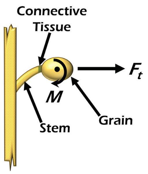
Engineers designing mechanisms to dissociate grain need to understand the basic principles of tensile and bending failure. Most grains are attached to the plant by some kind of stem and/or connective tissue. The connective tissue can often be understood as a cylindrical bundle of connective tissue. Most dissociation mechanisms apply a tensile force, a bending force, or a combination of the two on the seed relative to the plant (Figure 3.3.2). The goal of the force application is to cause a failure of the connective tissue between the grain and the stem or plant. Failure will occur when the stress in the connective tissue exceeds its ultimate yield stress, which is the stress at which the material will break. Obviously, it is desirable for the dissociation failure to occur as close to the individual grain as possible so that there is no stem or other plant material captured with the grain.

Figure \(\PageIndex{2}\): Dissociation forces acting on a grain. F_t is the tensile force and M is the bending force, or moment.

Tensile failure is the mode where the grain is pulled straight away from the stem until the connection fails. The linear tensile force induces stress in the connective tissue that can be calculated by the following equation:

\[ \sigma_{t} = \frac{F_{t}}{A} \]

where σ_t = tensile stress in the connective tissue measured in force per unit area (N m⁻²)

F_t = tensile force acting on connective tissue (N)

A = cross-sectional area of the connective tissue (m²)

Bending failure occurs when the grain is rotated relative to the stem inducing bending stress in the connective tissue. Bending force or moment (M) can also be thought of as a rotational torque applied to the grain. Bending stress is described by the following equation:

\[ \sigma_{b} = \frac{M_{y}}{I} \]

where σ_b = bending stress in the connective tissue measured in force per unit area (N m⁻²)

M = bending force acting on the connective tissue measured in force × distance (N m)

y = perpendicular distance to neutral axis (m)

I = area moment of inertia of the connective tissue cross section in units of length to the fourth power (m⁴)

The moment of inertia is a quantity that is based on the shape of the cross section of the member and is used to characterize the member’s ability to resist bending.

Bending stress is a bit more complicated than tensile stress because the stress in the member is not constant across its cross section. Fibers farther from the neutral axis of bending will experience higher stress, which can actually enhance dissociation.

One of the challenges with describing failure of plant materials mathematically is the wide variability that can occur. The strength of the connective tissue is affected by three main factors based on biological properties of the plant. The first factor is plant size. Some plants within a single crop may grow larger than others and may have more connective tissue between the stem and grain. This would correspond to larger area and moment of inertia in Equations 3.3.7 and 3.3.8, which would require more force to reach the ultimate stress.

The second factor affecting connective tissue strength is plant maturity. Most plants will lose their grains naturally when they reach maturity as a mechanism for propagation. Mathematically, this natural dissociation is described by a reduction in the yield strength of the connective tissue. Quite often, this natural maturity state corresponds with the optimum time for grain harvest; however, it is not always possible to harvest at that exact time. Therefore, the failure strength could vary significantly based on actual harvest time.

The third factor affecting the strength of the connective tissue is moisture content. The strength properties of plant material vary greatly with moisture content. Engineers need to understand a number of biological properties of the plant as they are affected by moisture content. For instance, the turgor pressure in a plant is the pressure exerted on the walls of the cells within the plant by the moisture in the cells. As turgor pressure decreases, which is caused by a reduction in moisture content, plants become less rigid. In some plants, this might weaken the plant structure, making dissociation easier, but in others it could make it more difficult to dissociate a grain because the plant material would be more elastic. Depending on weather conditions and solar intensity, turgor pressure can vary greatly throughout a single day, affecting the dissociation of the crop.

Further complicating the mathematical representation of plant strength is the fact that there can be significant variability of plant size, maturity, and moisture content between different regions of a field, between different plants, and even between different grains on a single plant. Engineers need to develop mechanisms that accommodate this variability and give machine operators the flexibility to adapt the machine to the various conditions.

Separation

Once the grains are dissociated from the plant, they must be separated from the rest of the plant material and any other undesirable material. This undesirable material is called material other than grain (MOG). The separation performance of a harvesting machine is quantified by the separation loss (L_s), which is the amount of free grain that cannot be separated from the MOG expressed as a percentage of the total amount of grain that was dissociated from the plants by the machine.

There are two main principles that are typically used to separate grain from MOG. The first is mechanical separation through sieving. A sieve is simply a barrier with holes of a correct size that allows the desired particles to pass through while preventing larger particles from passing, or vice versa, allow smaller undesirable particles to pass through while retaining the desired particles. Some grain sieving mechanisms rely on gravitational forces on the particles to cause them to pass downward through the sieve openings; others utilize centripetal forces of rotating mechanisms to force particles outward through the sieves. Most gravitational sieving mechanisms induce a shaking or bouncing motion on the material to enhance the separation process by facilitating particle motion downward through the mat of material as well as causing motion of the material across the sieve.

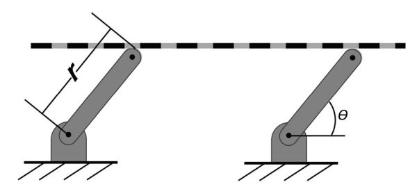
Consider the sieve plate connected to the parallel rotating bars as shown in Figure 3.3.3. This is a classic four-bar linkage mechanism. The sieve plate moves in a circular pattern while maintaining its horizontal orientation. If the design of the length of the rotating arms along with the rotational speed is correct, the material is bounced laterally across the plate. As it bounces, the grains move downward through the mat of material, then through appropriately-sized holes in the plate. The MOG travels across the plate and is deposited off the end of the sieve.

Figure \(\PageIndex{3}\): Simple sieve mechanism.

The velocity of the sieve plate (v) can be calculated from the following equation:

\[ v = r\omega \]

where v = velocity of the sieve plate (m s⁻¹)

r = length of the rotating support, or connecting, arms (m)

ω = rotational speed of the arms (radians s⁻¹)

The velocity of the sieve plate is actually the tangential velocity of the rotating support arms. The direction of this velocity changes sinusoidally as the bars rotate. The vertical (v_v) and horizontal (v_h) components of the velocity can be described with the following equations:

\[ v_{v} = v\ cos\theta \]

where θ = the angular position of the arms.

The bouncing motion of a particle is analyzed by considering the momentum of the particle in relation to the upward moving, but decelerating, plate to determine if and when the particle will leave the plate.

The second principle that is used to separate grains from MOG is aerodynamic separation. Quite often, the grain particles are denser and have significantly different aerodynamic properties than the MOG, especially the lighter leaf and hull particles. These differences are exploited to separate the MOG from the grain.

Figure \(\PageIndex{4}\): Forces affecting particle motion when it is free falling (left) and when subjected to a directed air flow (right).

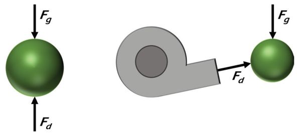
A particle that is moving through any fluid, including air, is subjected to gravity and drag forces (Figure 3.3.4). Gravity acts downward on the particle and produces the force represented by:

\[ F_{g} = mg \]

where F_g = gravitational force (N, or m kg s⁻²)

m = mass of the particle (kg)

g = gravitational constant in units of length per unit time squared (9.81 m s⁻²)

The drag force acts in the opposite direction of the particle’s motion relative to the air. The drag force is calculated by:

\[ F_{d} = 0.5\rho_{air}v^{2}_{part}C_{d}A_{part} \]

where F_d = drag force (N, or m kg s⁻²)

ρ_air = density of the air in units of mass per unit of volume (kg m⁻³)

v_part = velocity of the particle relative to the air in units of length per time (m s⁻¹)

C_d = unitless drag coefficient of the particle

A_part = characteristic area of the particle (m²).

The motion of the particle is determined by the vector sum of the two forces and the fundamental motion equation:

\[ a = \frac{F_{r}}{m} \]

where a = acceleration of the particle in the direction of the resultant force (m s⁻²)

F_r = resultant force on the particle (N, or m kg s⁻²)

The particle trajectory can be described mathematically by integrating the acceleration equation once to get the velocity equation, then a second time to find position as a function of time.

The drag coefficient is a function of many particle factors including its shape and surface texture. Many MOG particles, such as seed hulls and stem particles, have a more irregular shape and surface texture than the grains and, thus, will have a higher drag coefficient. Aerodynamic separation occurs by capitalizing on these drag differences as well as differences in mass between the grain and MOG particles. Particles can be separated if an air stream is directed through the mat of grain and MOG in such a manner that the MOG is directed in a different trajectory than the grains.

Consider an air stream created by a fan blowing straight upward at a falling particle. If the air speed is increased to the point that the drag force equals the gravity force, the particle will be suspended in the air stream. The velocity of the air at this point is, by definition, the terminal velocity of the particle. If the air speed is increased, the particle will move upward; if the air speed is decreased, the particle will move downward.

Consider a mixture of grain and MOG particles being dropped through a directed air stream as illustrated in Figure 3.3.4. If the air velocity is set slightly below the terminal velocity of the grains, their trajectory will be altered to the right somewhat, but they will continue to move downward. MOG particles that have a much higher drag force and correspondingly lower terminal velocity will be carried more upward and to the right by the air stream moving them out of the grain flow.

Transport

Once the grain is dissociated and separated from the MOG, it must be transported to a receiving station. This is usually accomplished in several steps or stages using a variety of mechanisms. Various types of conveyors are used to move the grain from one part of a machine to another or from one machine to another. At different stages of the process, the grain might be stored or carried in various bulk containers.

The principles involved with designing or analyzing bulk storage or transportation containers are primarily strength of materials. The designer first needs to determine what forces will be produced on the structure by the grain. Free body diagrams are analyzed to determine the magnitude and direction of all forces. One challenge in designing grain harvesting machinery is that the machines are often mobile. As the machines move across the rough terrain typically encountered in agricultural fields, dynamic forces are induced as the grain load bounces. Designers typically utilize a variety of techniques to predict the maximum dynamic loads that could be induced on a structure.

Once the forces are known, the designer then determines what stresses are induced in each structural member by the grain load. Stress (σ) describes the amount of force (F) being carried per unit area (A) of a given structural member:

\[ \sigma = \frac{F}{A} \]

where σ = stress in units of force per unit area (N m⁻²)

F = force in the member (N)

A = characteristic area of the member (m²)

The stress in any part of a structural member cannot exceed the yield stress of the material or permanent damage (deformation) will be incurred. But even if permanent deformation is not induced in a structural member, engineers still need to be concerned about how much a structural member flexes or deflects. The deflection in a member is calculated from strain, which is:

\[ \epsilon = \frac{dL}{L} = \frac{\sigma}{E} \]

where ε = strain (dimensionless)

L = length of the member (m)

E = modulus of elasticity reported in force per unit area (N m⁻²)

Stress and strain are related by the modulus of elasticity, also known as Young’s modulus. The lower the modulus of elasticity, the more deflection a given force will cause in a member. Some deflection can be good in a structure, especially when dynamic forces are involved, because it helps to absorb energy without causing high peak loads. In the case of a machine moving across a rough field, for example, some deflection in the structure can absorb some of the energy caused by uneven terrain and prevent structural failure.

For shorter distance transportation, several different conveying devices can be employed. When designing conveying devices, the designer is primarily concerned about the capacity of the device and the power required to convey the material. Some of the simplest conveying devices utilize paddles or buckets connected to chains (Figure 3.3.5) to drag or convey the grain. The capacity of paddle conveyors, which is the flow rate of material through the conveyor, is calculated simply by the amount of material carried by each paddle and the number of paddles that pass a point in a given amount of time:

\[ Q_{a} = Vn \]

Figure \(\PageIndex{5}\): Simple paddle conveyor.

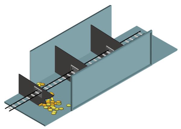
where Q_a = actual flowrate in volume per unit time (m³ s⁻¹)

V = volume of material carried by a single paddle (m³)

n = number of paddles that are discharged per unit time (s⁻¹)

The volume of material that can be carried by the paddles is affected by a number of parameters. Grain properties such as particle shape, size, surface friction and moisture content affect the shape of the pile of grain on each paddle. The slope of the conveyor limits the size of the piles before the grain runs over the top of the paddle and back down the conveyor.

Figure \(\PageIndex{6}\): Simple screw conveyor.

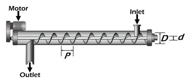
Another conveying device commonly used in grain harvest and handling is a screw conveyor, commonly known as an auger (Figure 3.3.6). Screw conveyors utilize a continuous helicoid plate, called flighting, attached to a rotating shaft. The capacity of a horizontal screw conveyor that is completely full of grain is the volume displaced by a single rotation of the shaft times the number of rotations in a given unit of time, which can be calculated by:

\[ Q_{t}=\frac{\pi}{4} (D^{2}-d^{2})P\omega \]

where Q_t = theoretical flowrate in volume per unit time (m³ s⁻¹)

D = outside diameter of the flighting (m)

d = diameter of shaft (m)

P = pitch length of the flighting (m)

ω = rotational speed of the shaft (radians s⁻¹)

When the conveyor is inclined, the flighting will no longer be full as the grain will tend to slide down around the flighting. The actual volumetric flowrate (Q_a) can be calculated by:

\[ Q_{a}= Q_{t} \eta_{v} \]

where η_v is the volumetric efficiency of the conveyor. Predicting the volumetric efficiency can be very challenging because it is affected by numerous factors, including conveyor slope, rotational speed, grain moisture content, particle size, particle to conveyor friction, and particle-to-particle friction. Because of this complexity, mathematical prediction is usually accomplished with empirical relationships.

The power required to convey the material is affected by gravitational and friction forces. If the grain is lifted any vertical distance, the conveyor must overcome the gravitational force opposing that lift. Power is defined as a force applied over a given distance in a given amount of time (force × distance/time). The force and time components of the gravitational power calculation come from the flow rate of the grain through the conveyor expressed in units of weight per unit of time. The density of the grain can be used to convert volumetric flow rate into a weight flow rate. The distance component of power is simply the vertical distance that the grain is lifted. The gravimetric component of power is:

\[ P_{q} = Q_{a}\rho_{grain}h \]

where P_g = power required to overcome gravity (W or J/s)

Q_a = actual volumetric flow rate of grain (m³ s⁻¹)

ρ_grain = density of the grain (kg m⁻³)

h = height that the material is lifted (m).

The friction component of power can be more complicated to compute. In the case of a paddle conveyor, the grain must be slid along the bottom of the conveyor surface. This friction force can sometimes be predicted quite well from the coefficient of friction between the grains and the surface of the conveyor. If that coefficient of friction gets too large, the forces due to friction on the grains at the interface between the grain pile and the conveyor surface will cause the grains within the pile to begin to move relative to each other. At this point, it becomes more difficult to mathematically describe the energy necessary to overcome these internal friction forces as well as the surface friction.

Frictional forces in screw conveyors are similar. The grain in a full horizontal conveyor slides along the outside wall of the conveyor tube as well as the flighting but does not move as much within the grain mass. As the conveyor is inclined and it is no longer completely full, the amount of motion within the grain mass increases and becomes more critical to the evaluation.

Applications

The most common machine used for grain harvest is the modern grain combine (Figure 3.3.1). Combines typically have an interchangeable attachment on the front called a header that engages the crop and passes certain fractions of that plant into the combine. The material then passes through a threshing mechanism that dissociates the grains from the plant stems and also performs some separation of grain from MOG. The grain and MOG are then passed through various separating and cleaning mechanisms. The MOG is generally passed longitudinally through the machine and expelled from the back. The clean grain generally moves downward through the machine to a catch reservoir on the bottom. From there, it is moved upward with paddle and/or screw conveyors to a holding tank on the top of the machine. A large screw conveyor is then used to periodically empty the contents of the holding tank into a truck or other vehicle, which transports the grain to a receiving station.

Engagement

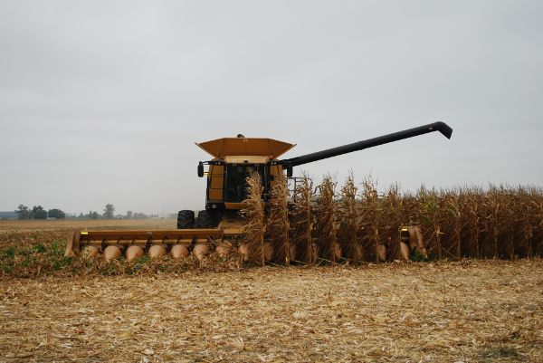
Header attachments are used to engage the crop. The two most common types of header attachments on grain combines are the grain table and the corn or row head. Grain tables (Figure 3.3.1) are typically used in small grain crops such as wheat and soybean. They generally include a large gathering reel to engage the crop and pull it into the header. A cutting mechanism, typically a sickle bar, cuts the plant as it is pulled into the header to gain mechanical control of the grain. Since grain tables can be 12 m wide or wider, cross conveyors move the crop material from the ends of the header to the center where it is fed into the combine.

The height of the cut depends on the crop and the cultural practice of the operation. The threshing and separation processes in the combine are most efficient when the MOG entering the combine is minimized. In soybean, for example, the seed pods can grow very low on the plant stem; therefore, the crop must be cut near the ground to prevent losses. In crops like wheat where the grains grow in a head on the top of the plant stem, the cut height could be just low enough to capture the entire head but minimize the amount of MOG passed into the machine. In some production systems, though, the MOG might be used for animal bedding or bioenergy. In these cases, the header is operated lower so that more MOG is gathered, passed through the combine and deposited in a narrow line, called a windrow, behind the combine. The windrow can easily be gathered by another biomass harvesting machine in a separate operation. Occasionally, the MOG is gathered by another machine, such as a baler, attached directly to the combine (Figure 3.3.7).

Figure \(\PageIndex{7}\): Combine with attached baler to collect biomass.

In corn (maize), the grains are produced toward the middle of the plant. Cutting the plant to capture the ears for threshing would mean the introduction of large amounts of MOG into the harvest stream, hampering threshing and separation performance. Since corn is typically grown in rows spaced 0.5–0.75 m, corn heads are constructed with fingers that pass between the rows so that each row of corn can be engaged individually (Figure 3.3.8). Long parallel rollers on each side of the row grab the plant stems below the ear and pull them downward as the machine moves forward. Stripper plates above each roller are spaced such that the plants pass down between them, but the corn ears do not. As the plants are pulled downward, the ears are stripped off the plants. Ideally, all of the plant material is pulled down through the header and does not pass into the combine. Depending on stalk condition, some stalk breakage and leaf removal will occur, and that MOG will have to be separated in the combine. Chains with fingers above each stripper plate move the ears and MOG back into the header. Cross conveyors then move material from the edge of the header into the center where it is fed into the combine.

Figure \(\PageIndex{8}\): Typical row-crop header on a combine.

One of the performance measures of any header is its effectiveness in gathering all of the grain from the field into the combine. This engagement process is complicated by the fact that the grains tend to naturally fall off of the plants more easily when the crop is in its optimum harvest condition. Losses by the header are called shatter losses (L_sh). They are quantified as a percentage of the potential yield (y_p), i.e., the available yield of the plants.

Shatter losses are affected by crop conditions, including maturity and moisture content. They are also affected by the design and operation of the header. For example, the speed of the gathering reel on grain tables must be matched to the forward speed of the machine. If the reel speed is too high, the plants are beaten aggressively, causing grains to fall off the plants before they can be caught on the header platform. If the reel speed is too slow, the plants could be pushed forward, again knocking grains onto the ground before they enter the header. Depending on crop conditions, the tangential speed of the reel is typically operated at least 25–50% faster than the forward speed of the combine to pull the plants into the header. Some machines utilize sensors and electronic controls to automatically adjust the reel speed to match machine forward speed.

Dissociation

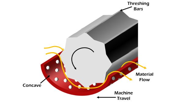
The dissociation function in combines is generally accomplished by rotating cylinders called threshing cylinders. There are two basic configurations of threshing cylinders, distinguished by the direction the material moves through the cylinder. Some cylinders are mounted with their axis of rotation horizontal and perpendicular to the longitudinal axis of the machine. The material enters from one side of the cylinder and exits the other (Figure 3.3.9). Bars oriented along the outside of the cylinder rub the plant material against the stationary housing around the outside of the cylinder, which is called the concave. The rubbing action affects the dissociation of the grain from the plants. Holes in the concave facilitate a sieving action to separate some of the grain from the longer plant material.

Figure \(\PageIndex{9}\): Transverse-mounted (conventional) threshing cylinder.

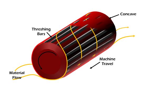
The other common threshing configuration has the rotating threshing cylinder mounted parallel to the longitudinal axis of the machine. Material enters the end of the cylinder and moves in a helical pattern around and past the cylinder (Figure 3.3.10). Similar concave structures around the cylinder provide resistance to the flow to induce the dissociation and separation functions.

Figure \(\PageIndex{10}\): Longitudinal-mounted (rotary) threshing cylinder.

Threshing effectiveness is measured by the percentage of grains that are dissociated from the plants, the percentage of grains that are damaged during the threshing process, and the amount of MOG break-up. Excess amounts of small MOG particles can hamper separation efficiency since they can be indistinguishable from grains in the separation process. Threshing efficiency and grain damage are affected by plant properties, the design of the cylinder and concaves, and operational adjustments. Machine operators often have real-time control of the cylinder speed as well as the clearance between the cylinder and concave.

Separation

There are two different types of separation systems used in grain combines that are generally associated with the two types of threshing devices. Laterally oriented threshing cylinders generally feed the material stream onto a vibrating separator platform commonly called a straw walker. The oscillating plate is essentially a sieve allowing the smaller particles, including the grains, to fall through the sieve as the MOG is moved back through the machine.

On combines with axially oriented threshing cylinders, the latter portion of the cylinder and concave accomplish initial separation. These rotary separators utilize centripetal forces to separate grains outward through concave openings.

Regardless of the initial separator configuration, most combines pass the grain stream captured from the threshing unit and initial separation unit through an additional multi-stage cleaning sieve. Pneumatic separation is also applied in these sieves to enhance separation of grain from MOG.

Transport

The cleaned grain stream is conveyed from the bottom of the combine to a holding tank on the top of the machine using a combination of paddle and screw conveyors. The holding tanks vary in size with the size of the machine. Depending on the crop and operating conditions, the combine tank could be filled in as little as 3–4 minutes. In some operations, the combine is driven to the edge of the field when the tank is full so that it can be emptied into a truck for transport to a receiving station. This is often considered an inefficient use of a very expensive harvesting machine. Productivity of the harvesting operation is maximized if the combine can be operated as close to continuously as possible.

Figure \(\PageIndex{11}\): Typical grain cart receiving clean grain from a combine.

Combines can be unloaded while they are harvesting if a receiving vehicle can be driven alongside the combine. Over-the-road trucks are not typically used for this operation because of their relatively small tires. Traction in potentially soft soil conditions limits their mobility. Also, there is a concern regarding compaction of the soil in the field. Heavy loads on small tires will compact the soil under the tires causing damage that will affect the performance of future crops in the field.

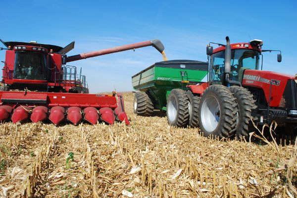
In-field transport of grain is often accomplished with a grain cart (Figure 3.3.11). Grain carts are large transport tanks typically pulled by large agricultural tractors. Both the cart and tractor will be equipped with large tires or tracks to reduce the pressure on the soil.

With the use of grain carts, a logistical challenge arises around the best way to get the grain away from the combine to keep it harvesting. Many operations use multiple combines in a field simultaneously. Managers must decide how many grain carts are needed, how big those carts need to be, and how many trucks are needed to get the grain away from the field. Operationally, vehicle scheduling is a challenge to anticipate which combines in a multiple combine fleet must be emptied so that they do not fill up and become unproductive.

Examples

Example \(\PageIndex{1}\)

Example 1: Combine harvest efficiency

Problem:

One way to evaluate the harvest efficiency of a combine is to measure losses that occur as a combine moves through the field. This can be done by physically gathering and counting or weighing the grains found at different locations in the combine’s operating space.

Consider the combine in Figure 3.3.12 that was stopped while harvesting a very uniform crop of wheat. Field measurements were taken at three different locations as shown. At each point, a 1 m square area was selected as a representative test area. At point A in front of the combine, all of the standing plants in the test area were carefully cut and hand harvested to determine how much grain was available in the field. After that, the grains that were laying on the ground in that test area were gathered and weighed. At point B, all of the grains found within the test area were gathered and weighed. At point C, which is beyond the discharge trajectory of material being expelled from the back of the combine when it was stopped, all of the grains were collected and weighed separately by those that were still attached to the plants and those that were free. The following are the data collected at each location.

Figure \(\PageIndex{12}\): Locations of performance test measurements for a grain combine harvesting wheat.

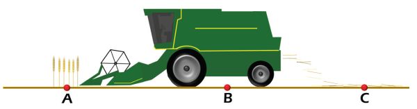
• Point A:
  • 335 g unharvested grain
  • 15 g free grains (grains laying on the ground)
• Point B:
  • 40 g free grain
• Point C:
  • 63 g free grain
  • 14 g grain attached to plant

Determine the gathering, threshing, and separating efficiencies of this harvest operation.

Solution

The theoretical or potential yield, y_p, of the crop is the harvestable grain that is still attached to the plants when the combine engages it. In this example, the potential yield is based on the unharvested seed at point A.

\( y_{p} = \frac{0.335 \text{ kg}}{\text{m}^{2}} \cdot \frac{10000 \text{ m}^{2}}{ \text{ha}} = \frac{3350 \text{ kg}}{\text{ha}} = \frac{3.35 \ T}{\text{ha}} \)

A simple unit conversion can be performed to convert the metric yield into common U.S. yield units of bu/acre as:

\( y_{p} = \frac{3350 \text{ kg}}{\text{ha}} \cdot \frac{1 \text{ bu}}{27.22 \text{ kg}} \cdot \frac{1 \text{ ha}}{ 2.47\text{ acre}} = \frac{49.8 \text{ bu}}{\text{ha}} \)

Note that the potential yield calculation does not consider the grains that had fallen from the plants before the machine engaged them. In this example, the pre-harvest yield loss, y_ph, was:

\( y_{ph} = \frac{0.015 \text{ kg}}{\text{m}^{2}} \cdot \frac{10000 \text{ m}^{2}}{\text{ ha}} = \frac{150 \text{ kg}}{\text{ha}} \)

As a percentage of the total available grain, the pre-harvest yield loss was:

\( L_{ph} = \frac{150}{3350 + 150} \cdot 100 = 4.3 \text{%} \)

The grain that was collected at point B under the combine includes the shatter losses as well as the pre-harvest losses. The pre-harvest losses are subtracted from the total grain at point B to determine grain lost as the header engaged the crop. The shatter loss, L_sh, is calculated as a percentage of the theoretical yield as follows:

\( L_{sh} = \frac{(40 \text{ g}-15 \text{ g})}{335 \text{ g}} \cdot 100 = 7.5 \text{%} \)

Threshing loss is a quantification of the grains that did not get dissociated from the plant. These grains are found at point C still attached to plant material. The threshing loss percentage is based on the total grain that actually enters the combine. In this example, the shatter loss is removed from the total available grain in calculating the threshing loss, L_th, as follows:

\( L_{th} = \frac{14 \text{ g}}{(335 \text{ g}-25 \text{ g})} \cdot 100 = 4.5 \text{%} \)

The separation loss is threshed grain that is not removed from the MOG stream and is lost out the back of the combine. The free grain collected at point C includes the separation loss as well as the shatter and yield losses. Therefore, the loss due only to separation, L_s, is:

\( L_{s} = \frac{(63 \text{ g} - 15 \text{ g} - 25 \text{ g})}{(335 \text{ g} - 25 \text{ g})} \cdot 100=7.4 \text{%} \)

The total harvest loss, L_h, is based on all the grain lost by the combine, which would be:

\( L_{h} = \frac{63 \text{ g} + 24 \text{ g} - 15 \text{ g}}{335 \text{ g}} \cdot 100 = 19\text{%} \)

The actual harvested yield, y_a, then, is:

\( y_{a} = \frac{3.35 \ T}{\text{ha}}- \frac{0.19(3.35 \ T)}{\text{ha}} = \frac{2.71 \ T}{\text{ha}} \)

The harvest efficiency is (Equation 3.3.6):

\( E_{h} = 1 -L_{h} = 1-0.19 = 0.81 \)

This can be verified by Equation 3.3.4:

\( E_{h} = \frac{y_{a}}{y_{t}} = \frac{2.71 \ T}{\text{ha}} \cdot \frac{\text{ha}}{3.35 \ T} = 0.81 \)

The prudent manager would scrutinize these harvest efficiency numbers to determine if improvements are merited. For wheat harvest, these losses would probably be considered quite large. The manager may consider adjustment and/or operational changes to the combine that might reduce harvest losses.

Example \(\PageIndex{2}\)

Example 2: Reel speed

Problem:

One of the causes of shatter loss with grain tables is improper speed of the reel. The designers of a grain table need to provide ample adjustability in the rotational speed of the reel so that the operator can compensate for crop conditions and forward speed. Specifically, the designer needs to determine the range of speeds that the design must be able to achieve. Consider the grain table in Figure 3.3.13 that has a 1.3 m diameter reel. Determine the range of reel speeds that the design must be able to achieve.

Figure \(\PageIndex{13}\): Gathering reel on grain table.

Solution

As mentioned earlier, the tangential speed of the engaging devices on the end of the reel should typically be 25–50% greater than the combine forward speed, v_f. ASAE Standard D497.7 is a great resource for operating parameters of common agricultural machinery. Table 3.3.3 of that standard (reprinted in part as Table 3.3.2 of this chapter) indicates that the typical forward speed of a self-propelled combine ranges from 3.0 to 6.5 km/hr. The minimum rotational speed of the reel would occur with the reel tangential speed 25% greater than the slowest forward speed of 3.0 km/hr. Conversely, the maximum speed would occur at 150% of 6.5 km/hr. The tangential speed, v_t, is calculated using Equation 3.3.9:

Table \(\PageIndex{2}\): Field efficiency and field speed for common harvesting machinery (excerpt from Table 3.3.3 in ASABE Standard D497.7, 2015b).

	Field Efficiency		Field Speed
Harvesting Machine	Range %	Typical %	Range mph	Typical mph	Range km/h	Typical km/h
Corn picker sheller	60–75	65	2.0–4.0	2.5	3.0–6.5	4.0
Combine	60–75	65	2.0–5.0	3.0	3.0–6.5	5.0
Combine (SP)	65–80	70	2.0–5.0	3.0	3.0–6.5	5.0
Mower	75–85	80	3.0–6.0	5.0	5.0–10.0	8.0
Mower (rotary)	75–90	80	5.0–12.0	7.0	8.0–19.0	11.0
Mower-conditioner	75–85	80	3.0–6.0	5.0	5.0–10.0	8.0
Mower-conditioner (rotary)	75–90	80	5.0–12.0	7.0	8.0–19.0	11.0
Windrower (SP)	70–85	80	3.0–8.0	5.0	5.0–13.0	8.0
Side delivery rake	70–90	80	4.0–8.0	6.0	6.5–13.0	10.0
Rectangular baler	60–85	75	2.5–6.0	4.0	4.0–10.0	6.5
Large rectangular baler	70–90	80	4.0–8.0	5.0	6.5–13.0	8.0
Large round baler	55–75	65	3.0–8.0	5.0	5.0–13.0	8.0
Forage harvester	60–85	70	1.5–5.0	3.0	2.5–8.0	5.0
Forage harvester (SP)	60–85	70	1.5–6.0	3.5	2.5–10.0	5.5
Sugar beet harvester	50–70	60	4.0–6.0	5.0	6.5–10.0	8.0
Potato harvester	55–70	60	1.5–4.0	2.5	2.5–6.5	4.0
Cotton picker (SP)	60–75	70	2.0–4.0	3.0	3.0–6.0	4.5

\( v_{t} = r \omega \)

At the minimum rotational speed, the tangential speed should be:

\( v_{t} = v_{f}(1.25) \)

Combining the equations, the minimum rotational speed is:

\( \omega = \frac{v_{t}}{r} = \frac{v_{f}(1.25)}{r} = \frac{3 \text{ km}}{\text{hr}} \cdot \frac{1.25}{1} \cdot \frac{2}{1.3 \ m} \cdot \frac{1000 \ m}{\text{km}} \cdot \frac{1 \text{hr}}{60 \text{ mins}} \cdot \frac{1 \text{hr}}{2\pi} = 15.4 \ \text{rpm} \)

It follows, then, that the maximum rotational speed is:

\( \omega =\frac{v_{t}}{r}=\frac{6 \text{ km}}{\text{ hr}}\cdot \frac{1.5}{1} \cdot \frac{2}{1.3 \ m} \cdot \frac{1000 \ m}{\text{km}}\cdot \frac{1 \ hr}{60 \text{ min}} \cdot \frac{1 \text{ rev}}{2\pi} = 36.7 \ rmp \)

The revolution units are added to the calculations by noting that radians are considered unitless, and there are 2π radians in one complete revolution. The conclusion is that the drive system for the reel on that grain table must be able to achieve speeds varying from 15.4 to 36.7 rpm, so the drive mechanism for the reel should be designed accordingly.

Example \(\PageIndex{3}\)

Example 3: Axle loads

Problem:

The design of the structure of a vehicle relies heavily on understanding the effects of all the forces on the machine. Consider a two-wheeled grain cart pulled by a tractor as shown in Figure 3.3.14. The task is to calculate the required size (diameter) of the cylindrical axles to support the cart wheel assembly. Assume that the grain load is evenly distributed in the tank of the cart and that the tank is laterally symmetrical, which means that the loads are evenly distributed between the left and right wheels of the cart. Besides the dimensions shown in Figure 3.3.15, the following data are given by a manufacturer for a very similar cart:

Figure \(\PageIndex{14}\): Basic grain cart pulled by an agricultural tractor.

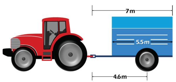
• Cart capacity: 850 bushels of corn (maize)
• Empty cart weight: 54 kN
• Tongue weight of empty cart: 11 kN

Solution

Because of the left/right symmetry of the cart, the free body analysis can be conducted in two dimensions looking at the side of the machine (Figure 3.3.15). The two cart wheels will have identical loads. Since the tractor supports 11 kN of the empty cart weight from the tongue at the hitch point (F_ct), the rest of the empty cart weight, which is 54 kN – 11 kN = 43 kN, must be supported by the cart wheels (F_cw). Given the symmetry and uniform loading assumptions, the center of gravity of the grain load will be at the geometric center of the bin on the cart. The distance from the hitch point to the grain center of gravity, x_g, is:

Figure \(\PageIndex{15}\): Free body forces acting on a grain cart.

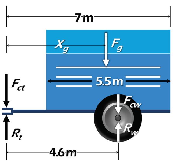
\( x_{g}= 7 - \frac{5.5}{2}=4.25 \ m\)

The weight of the grain is:

\( F_{g}=\frac{850 \text{ bu}}{1} \cdot \frac{25.4 \text{ kg}}{\text{bu}} \cdot \frac{9.81 \text{ N}}{\text{ kg}} = 212 \text{ kN} \)

The cart and grain must be supported by the cart wheels and by the tractor at the hitch point. These forces are represented as reaction forces R_w and R_t (Figure 3.3.15). R_w is the total weight that the cart wheels and axles must support, which can be calculated by summing the moments about the hitch point between the cart and tractor. If counter-clockwise rotation is positive, that moment equation is:

\( R_{w}(4.6) - F_{cw}(4.6) - F_{g}(4.25) + F_{ct}(0)-R_{t}(0) = 0 \)

Note that because the tongue load and reaction force both pass through the hitch point; their moment arm distances are zero and they fall out of the equation. The moment equation is now solved for R_w:

\( R_{w} = \frac{F_{cw}(4.6 \text{ m}) + F_{g}(4.25 \text{ m})}{4.6 \text{ m}} = \frac{43 \text{ kN}(4.6 \text{ m}) + 212 \text{ kNn}(4.25 \text{ m})}{4.6 \text{ m}} = 240 \text{ k} \)

Since there are two wheels, each wheel must support 120 kN.

With the load known, it is possible to calculate the diameter of the cylindrical axle required to support the wheel. The axle (Figure 3.3.16) is a cantilever configuration since it is rigidly fixed to the frame on one end. The simplified configuration of the axle (Figure 3.3.16) shows that the reaction force from the wheel is applied 30 cm out from the base of the axle. The downward force of the cart and grain at the base of the axle and the upward reaction force from the tire will cause bending stress in the axle. The bending moment is:

Figure \(\PageIndex{16}\): Configuration of axle on grain cart.

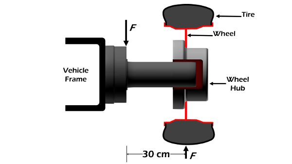
\( M=Fd=120,000 \text{ N }\cdot 0.3 \text{ m}= 3600 \text{ Nm} \)

The maximum stress in the axle cannot exceed the yield stress of the material, which would cause permanent deformation in the axle, compromising its functionality and strength. The designer needs to know what material will be used to manufacture the axle and then determine the yield stress for that particular material. A number of material engineering handbooks and other resources can be consulted to find the yield stress of different materials. For this example, assume that mild steel would be used. The yield stress for mild steel (σ_y) can be found from a number of resources to be 250 MPa. Note that a Pa is defined as a N/m². The bending stress in the axle is (Equation 3.3.8):

\( \sigma_{b} = \frac{My}{I} \)

Note that y is the distance from the neutral axis, which is the center of the circular shaft. The maximum stress will occur at the top and bottom of the axle. The equations for moment of inertia for different cross-sectional shapes can be found in a number of engineering handbooks or strength of materials text books. For a circular cross section, the moment of inertia is:

\[ I = \frac{1}{4} \pi r^{4} \]

Substituting Equation 3.3.21 into Equation 3.3.8, the bending stress equation becomes:

\( \sigma_{b} = \frac{4My}{\pi r^{4}} \)

Since the critical failure point will be at the outermost fibers of the circular cross section, the stress will be calculated at y = r. Also, the stress at those outermost fibers should not exceed the yield stress; therefore,

\( \sigma_{y} = \frac{4M}{\pi r^{3}} \)

Now solve for r:

\( r^{3}=\frac{4M}{\pi \sigma_{y}} \ \cdot \frac{3600 \text{ Nm}}{1} \ \cdot \frac{m^{2}}{350 \times 10^{6} \text{ N}} \)

The calculated minimum radius is 2.6 cm.

Any calculated number or computer output should always be scrutinized to make sure that it represents a reasonable conclusion. In this case, an experienced engineer should be concerned that a 2.6-cm radius axle seems unusually small for a large grain cart. There are several factors that were not considered in the analysis. First, the load on the axle was the static weight of the cart and grain. There was no consideration for peak dynamic loads that would be induced as the vehicle moved across the terrain of a farm field. The dynamic analysis would also need to consider fatigue stress in the material due to repeated loading. There was no safety factor considered to compensate for inconsistencies in material properties of the axle or overloading of the cart by the operator. Depending on the method of attachment of the axle to the frame, there could be significant stress concentrations at sharp corners or weldments. These stress concentrations are usually identified with a finite element analysis of the structure. But even if catastrophic failure did not occur in the mechanism, the engineer should consider the effects of the elasticity of the axle. In this case, excessive elastic deflection in the axle could cause the tire to become misaligned, which could cause adverse tracking of the cart or unacceptable wear of the tire. All these factors would need to be addressed to achieve a final design that prevents failure and assures proper operation.

Image Credits

Figure 1. Stombaugh, T. (CC By 4.0). (2020). Typical grain combine.

Figure 2. Stamper, D. & Stombaugh, T. (CC By 4.0). (2020). Forces acting on grain.

Figure 3. Stamper, D. & Stombaugh, T. (CC By 4.0). (2020). Simple sieve mechanism.

Figure 4. Stamper, D. & Stombaugh, T. (CC By 4.0). (2020). Drag forces.

Figure 5. Stamper, D. & Stombaugh, T. (CC By 4.0). (2020). Paddle conveyor.

Figure 6. Stamper, D. & Stombaugh, T. (CC By 4.0). (2020). Screw conveyor.

Figure 7. Stombaugh, T. (CC By 4.0). (2020). Combine and baler.

Figure 8. Stombaugh, T. (CC By 4.0). (2020). Row crop head.

Figure 9. Stamper, D. & Stombaugh, T. (CC By 4.0). (2020). Conventional threshing cylinder.

Figure 10. Stamper, D. & Stombaugh, T. (CC By 4.0). (2020). Rotary threshing cylinder.

Figure 11. Stombaugh, T. (CC By 4.0). (2020). Combine and grain cart.

Figure 12. Stamper, D. & Stombaugh, T. (CC By 4.0). (2020). Combine test locations.

Figure 13. Stamper, D. & Stombaugh, T. (CC By 4.0). (2020). Gathering reel.

Figure 14. Stamper, D. & Stombaugh, T. (CC By 4.0). (2020). Tractor and grain cart.

Figure 15. Stamper, D. & Stombaugh, T. (CC By 4.0). (2020). Forces on grain cart.

Figure 16. Stamper, D. & Stombaugh, T. (CC By 4.0). (2020). Axle configuration.

References

ASABE Standards. (2015a). ASAE EP496.3 FEB2996 (R2015): Agricultural machinery management. St. Joseph, MI: ASABE.

ASABE Standards. (2015b). ASAE D497.7 MAR2011 (R2015): Agricultural machinery management data. St. Joseph, MI: ASABE.

Srivastava, A. K., Goering, C. E., Rohrbach, R. P., & Buckmaster, D. R. (2006). Engineering principles of agricultural machines (2nd ed.). St. Joseph, MI: ASABE.