4.2: Water Quality as a Driver of Ecological System Health

Leigh-Anne H. Krometis

Biological Systems Engineering

Virginia Tech

Blacksburg, Virginia, USA

Key Terms

Water pollution	Source control	Water quality standards
Ecological and ecosystem services	Delivery control	Nutrient management
Pollutant budget	Assimilative capacity	Urban stormwater planning

Variables

• μ = viscosity of water
• ρ_p = density of particle
• ρ_w = density of the fluid (water)
• b = benefit
• BCR = benefit to cost ratio
• c = cost
• d = particle diameter
• D = depth
• g = acceleration due to gravity
• L = length
• M_in = mass of pollutant entering the system of interest (e.g., field, structure)
• M_out = mass of pollutant leaving the system of interest (e.g., field, structure)
• MOS = margin of safety
• NPS = nonpoint source contributions of the targeted pollutant
• PS = point source contributions of the targeted pollutant
• Q = inflow rate
• Q_R = overflow rate
• ∆S = mass of pollutant retained or treated by the system of interest (e.g., field, structure)
• TMDL = maximum permissible total quantity of targeted pollutant that can be added to the receiving water each day
• V_y = average vertical (“fill”) velocity
• V_s = settling velocity
• W = width

Introduction

Water is critical to all known forms of life, human and non-human. Poor management of water resources can result in risks to human health through the spread of toxic chemical and pathogenic microorganisms, reduction in species diversity through changes in water chemistry and/or habitat loss, economic hardship due to a failure to meet industrial, agricultural, and energy needs and political conflict or instability as neighboring states or nations struggle to equitably distribute water to their people.

Globally, 70% of freshwater withdrawals are used by the agricultural sector (World Bank, 2017). It is important to recognize, however, that these consumptive values can vary considerably by nation or global region depending on the local population size, ecology, climate, and primary industries present. In the United States, the U.S. Geological Survey (USGS) estimated that in 2011, 41% of consumptive water use (water that is not returned quickly to the same source from which it was taken) was devoted to hydroelectric power generation, 40% was used to support various forms of agriculture (aquaculture, livestock, crop irrigation), 13% supported domestic household use, and the remaining 6% was used for industrial purposes or in extractive industries (e.g., mining) (USGS, 2018). In contrast, the United Nations Food and Agriculture Organization (UNFAO) estimated in 2015 that over 64% of water in China and nearly 80% of water in Egypt supported agriculture (UNFAO, 2019). Although per capita water use has declined in recent years, the human population and its attendant need for clean water, affordable energy, and nutritious food continues to increase. Concurrently, non-human species diversity continues to decline as forest, soil, and water resources are increasingly exploited (MEA, 2005; Raudsepp-Hearne et al., 2010). More explicit consideration of the intricate feedback of food-energy-water systems within human populations and their impacts on other ecological services are needed to ensure sustainability.

This chapter introduces basic concepts related to water management and provides examples of best management practices that can be used to preserve and improve water quality. Here, we define ecosystem health as the capacity of a natural system to support human and non-human needs. In this chapter particular focus is on chemical, microbial, and physical constituents in water as drivers of ecosystem health.

Outcomes

After reading this chapter, you should be able to:

• • Define pollution in terms of assimilative capacity and use of water body
• • Explain the concept of ecological, or ecosystem, services and their relationship to water quality
• • Describe strategies for water pollution control, including pollutant budgets and stormwater best management practices
• • Calculate a range of water quality impairment and cost parameters

Concepts

Definition and Description of Water Pollution

The U.S. Environmental Protection Agency defines water pollution as “human-made or human-induced alteration of chemical, physical, biological, and radiological integrity of water” (USEPA 2018a). These alterations include the addition of specific pollutants (e.g., chemicals, microorganisms, sediment) to an aquatic system or the alteration of natural conditions, such as pH or temperature. In this context, the “integrity” of the water refers to the ability of the water to continue to perform appropriate human or ecological functions. These functions are spelled out explicitly by the European Environment Agency’s definition of pollution as “the introduction of substances or energy into the environment, resulting in deleterious effects of such a nature as to endanger human health, harm living resources and ecosystems, and impair or interfere with amenities and other legitimate uses of the environment” (EEA, 2019). While the two definitions are similar, it is critical to note that the EEA does not specify that pollution needs to be human-made.

A place where pollutants directly enter a receiving water such as a stream, river, or lake through an identifiable pipe or culvert (e.g., industrial outfall or wastewater treatment plant effluent) is referred to as a point source (PS) of pollution. Point sources are generally reasonably constant in flow and concentration (i.e., the pattern, type, and amount of pollution being discharged is consistent), because they tend to be governed by predictable or controlled processes. Places from which pollutants are transported to receiving waters via stormwater runoff (e.g., eroded sediment from construction sites and leachate from septic drainfields), or are more diffuse and less predictable in nature, are referred to as nonpoint sources (NPS) of pollution. NPS pollution is sometimes referred to as diffuse pollution, as the sources are distributed throughout the catchment, rather than originating from a distinct location. NPS discharges are generally highly variable and much more severe following significant weather events such as rainfall or seasonal events such as snowmelt. Consequently, NPS pollution is often more serious during high flows when greater quantities of pollutants are being transported to receiving waters, while PS pollution is more serious during low flows when there is less dilution of constant discharges (Novotny, 2003).

Although any changes to water through PS or NPS contributions may meet the technical definition of pollution, pollution is only considered a concern if it exceeds the receiving water’s waste assimilative capacity so that the water no longer supports its human or ecological purpose. Waste assimilative capacity is defined as the natural ability of a water body to absorb pollutants without harmful effects. Receiving waters can naturally process some level of pollution through dilution, photodegradation, and bioremediation. For example, native aquatic plants use nutrients including nitrogen and phosphorus to grow; however, very high nutrient contributions from anthropogenic sources can stimulate algal overgrowth, leading to harmful blooms, eutrophication and aquatic ecosystem collapse (Withers et al., 2014).

Ecological Services and Water Quality Decisions

Historically, human and ecological uses of water resources were sometimes regarded as separate or even competing aims. There is an increasing effort to acknowledge the inherent linkages and interdependence of human and ecological well-being through the concept of ecological, or ecosystem, services. Rather than promoting conservation of habitat and non-human species diversity solely for the sake of nature, the concept of ecological services recognizes that preservation and restoration of natural ecosystems also protects functions that ensure the sustainability of human communities. Ecological or ecosystem services are classified into four categories: regulating services (climate, waste, disease, buffering); provisioning services (food, fresh water, raw materials, genetic resources); cultural services (inspiration, spiritual, recreational, educational, scientific); and supporting services (nutrient cycling, habitats, primary production). Making ecological services (such as supporting fish populations, carbon sequestration, nutrient cycling, and flood mitigation) explicit allows for their quantification and inclusion in cost-benefit analyses associated with future land use planning and the allocation of funds for water quality improvements (Keeler et al., 2012; APHA, 2013; Hartig et al., 2014). Continuing research aims to uncover and quantify additional linkages between human health and well-being and ecosystem integrity, including promotion of mental health and community cohesiveness (Sandifer et al., 2015). This is in keeping with the mission of the American Society of Agricultural and Biological Engineers, whose members “ensure that we have the necessities of life: safe and plentiful food to eat, pure water to drink, clean fuel and energy sources, and a safe, healthy environment in which to live” (ASABE, 2020).

Designated Uses and Water Quality Standards

Water quality standards vary around the world. In some jurisdictions (e.g., countries, regions), minimum water quality standards are set for all water bodies regardless of use; in other jurisdictions, appropriate levels of different water quality constituents are generally determined based on chosen, intended, or planned uses of a water body. For example, in the U.S., states, tribes, and territories assign “designated” uses to surface waters to protect human health following water contact (e.g., drinking water reservoirs, recreation, fishing), to preserve ecological integrity (e.g., trout stream, biological integrity), and for economic or industrial use (e.g., navigation, sufficient flow for hydroelectric power). Acceptable levels of critical pollutants are then established to ensure the water body can continue to meet these designated uses. For instance, a water body used only for irrigation may have concentrations of nitrate (NO₃⁻), a soluble form of an important plant nutrient, that exceed safe levels for drinking water, without interfering with its use as irrigation water. Basing water quality standards on the designated use of the water body allows for these differences in quality requirements by use category to be taken into account.

An Example of Water Pollution Regulation: U.S.A.

The U.S. Clean Water Act, introduced in 1972, remains the primary regulatory mechanism to ensure surface waters in the U.S. continue to meet the designated uses while protecting human and ecological health. At its most basic, the Clean Water Act regulates point sources through the National Pollutant Discharge Elimination System (NPDES), which requires permits for discrete discharges to ensure implementation of best practicable technology and appropriate monitoring.

NPS pollution is primarily regulated through the Total Maximum Daily Load (TMDL) program, which requires states to monitor surface water and compile lists of waters that do not meet standards applicable for their designated uses, which are then classified as impaired and require TMDL development (Keller and Cavallaro, 2008; USEPA, 2019). The acronym TMDL has two distinct definitions: (1) the mathematical quantity of a targeted pollutant that a receiving water can absorb without harmful effects (Equation 4.2.1); and (2) the restoration process developed to bring that water body back into compliance with water quality standards (Freedman et al., 2004). Through this restoration process, acceptable levels of pollutant discharges are identified that will not exceed the waste assimilative capacity of the water body so that it can maintain pollutant levels appropriate to its designated use. Mathematically, TMDL is defined as:

\[ TMDL = PS + NPS+MOS \]

where TMDL = maximum permissible total quantity of targeted pollutant that can be added to the receiving water each day (mass day⁻¹)

PS = all point source contributions of the targeted pollutant (mass day⁻¹), regulated through the NPDES process

NPS = all nonpoint source contributions of the targeted pollutant (mass day⁻¹)

MOS = a margin of safety (mass day⁻¹)

TMDL is calculated on a load (mass) basis, e.g., mg day^-1, and for each individual pollutant that is compromising the use of the water body in question. Margins of safety are included to account for future land development, changes in climate, and uncertainties in measurements and modeling used in TMDL development. Once a total maximum daily load is determined for a water body to meet the relevant water quality standards (including how much pollutant can be allowed from PS and NPS), then treatment systems and land use changes can be designed to meet that maximum daily load.

Determining the allowable total maximum daily load combines mass balance and concentration information, which are described in more detail later in this chapter. While this calculation is simple, the most important part of solving the problem is keeping track of units and identifying the necessary data and information needed to complete the task. Occasionally, there may be an abundance of data but not all of it is valuable to the engineer, thus it is essential for an engineer to master the skills to identify exactly what data are needed to complete the calculation.

Engineering Strategies for Water Quality Protection

Strategies to preserve surface water integrity from degradation or to address water quality impairments are often referred to collectively as best management practices (BMPs). The USEPA defines a BMP as “a practice or combination of practices determined by an authority to be the most effective means for preventing or reducing pollution to a level compatible with water quality goals” (USEPA, 2018b). This term is more broadly encompassing than the National Academies’ Stormwater Control Measure (SCM), which primarily refers to structural practices implemented in urban areas to intercept stormwater (NRC, 2009). In addition to structural practices, the term BMP can be used to describe non-structural efforts to protect water quality, including public participation, community education, and pollutant budgeting, and is used to describe these efforts in a variety of land-water environments, including urban, agricultural, and industrial (e.g., mining, forestry) landscapes.

Water quality protection strategies can be broadly categorized as implementing either source control or delivery control. The function of many strategies for water quality protection can be described very simply using a mass balance:

\[ M_{in} = \Delta S + M_{out} \]

where M_in = mass of pollutant entering the system of interest (e.g., field, structure) (kg)

∆S = mass of pollutant retained or treated by the system of interest (kg)

M_out = mass of pollutant leaving the system of interest (kg)

This simple relationship is the foundation for the design, performance evaluation, and costing of BMPs. Application of Equation 4.2.2 to different types of strategies is described in the following sections.

Source Control

Source control refers to efforts to reduce the presence or availability of the pollutant in the land-water system (e.g., eliminating pesticide use) or to prevent transport of the pollutant from its original source (e.g., discouraging erosion by managing tillage in a field). Widespread use of chemical fertilizers has facilitated a more than doubling of cereal grain production globally over the past 50 years, allowing for the feeding of an ever-increasing population (Tilman et al., 2002). However, overuse of fertilizers can lead to nutrient losses via runoff to surface water and/or leaching to groundwater following precipitation events if soil amendments are not applied via an appropriate method at the time of year best suited to promote plant growth. Excessive nutrient loadings can result in eutrophication and aquatic biology impairments, as well as difficulty in meeting municipal drinking water needs. Use of fertilizers in excess of crop needs also represents an unnecessary and nontrivial expenditure for the producer. When applied to a source control practice such as nutrient management, the variables in Equation 4.2.2 are defined as:

M_in = mass of nutrient applied to the crop

∆S = mass of nutrient taken up by the crop + mass of nutrient adsorbed by the soil

M_out = mass of nutrient leaving the field in runoff, lateral flow through the soil, and in deep seepage.

Delivery Control

Delivery control refers to efforts to reduce pollutant movement to source waters after pollutants are moved from their point of origin. Often, delivery control efforts involve interception, treatment, and/or storage of pollutants in water (e.g., riparian buffer, detention basin) prior to their discharge into a receiving water. When applied to a source control practice such as a detention basin, the variables in Equation 4.2.2 are defined as:

M_in = mass of pollutant in inflow

∆S = mass of pollutant treated or retained

M_out = mass of pollutant in outflow

An example of delivery control is a detention basin in which runoff water is collected and the particles are allowed to settle out before the water flows out of the basin. A detention basin can be placed at the outlet of a watershed in which soil erosion is occurring (the NPS) to reduce the mass load of sediment flowing out of the watershed as part of a plan to meet the TMDL. Theoretical particle removal by size class in the detention basin can be calculated by assuming a theoretical stormwater basin of depth D, width W, and length L (Figure 4.2.1):

Figure \(\PageIndex{1}\): Theoretical stormwater basin dimensions.

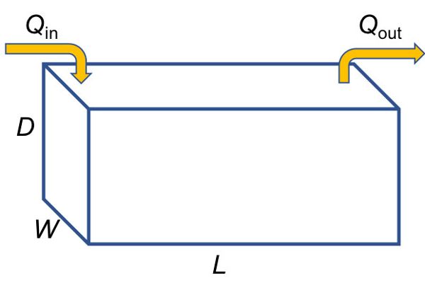
Assuming a constant inflow rate of Q, the average vertical (“fill”) velocity is approximated as flow divided by cross-sectional area of the basin, or:

\[ V_{y} = \frac{Q}{W \times L} \text{ for depth of water in the basin <D} \]

where V_y = average vertical (“fill”) velocity (m h⁻¹)

Q = inflow rate (m³ h⁻¹)

W = width (m)

L = length (m)

When the basin is full of water and inflow continues, water will flow out of the basin, and:

\[ Q_{R} = \frac{Q}{W \times L} \text{ when depth of water in the basin = D} \]

where Q_R = overflow rate (m h⁻¹)

Under laminar flow conditions (smooth flow at low velocity), the theoretical rate at which a particulate will settle from the runoff water is governed by Stokes’ law:

\[ V_{s} = \frac{gd^{2}(\rho_{p} - \rho_{w})}{18\mu} \]

where V_s = settling velocity (m s⁻¹)

ρ_p = density of particle (kg m⁻³)

ρ_w = density of the fluid (water), (kg m⁻³)

g = acceleration due to gravity (m s⁻¹ s⁻¹)

d = particle diameter (m)

μ = viscosity of water, 10⁻³ N s m⁻² at 20°C

Equations 4.2.3 and 4.2.5 can be used together to determine dimensions of the basin that will allow even small and light particles, such as fine silts, to settle to the bottom of the basin for a given inflow rate. Notice that both Equations 4.2.3 and 4.2.5 represent a velocity in the vertical direction; Equation 4.2.3 describes the change in water depth over time as the inflow fills the basin, and Equation 4.2.5 describes the vertical velocity of the particles in the water. When these are equal to each other, the dimensions of the basin are sufficient to allow the sediment particles to settle to the bottom of the basin before the now-clean water begins to leave the basin from the top (Figure 4.2.1). Detention basins can be sized to completely remove particles of a minimum size and density by setting overflow rate (Equation 4.2.4) equal to the theoretical settling velocity for that design size particle, e.g.:

\[ Q_{R} = \frac{Q}{W \times L} = \frac{gd^{2}(\rho_{p}-\rho_{w})}{18\mu} \]

Given a design inflow rate Q, and size and density of the small particles carried in with the flow, combinations of W and L (the dimensions of the basin) can be found that will accomplish the objective of settling the small particles to the bottom. This reduces the load carried in the outflow, reducing the consequences of sediment pollution downstream and helping to meet targets for maximum allowable load.

Cost-Benefit Analysis

Cost-benefit analysis (CBA) at its simplest uses an estimate of the monetary value of the benefits of a project (b, any currency, e.g., $ or €) divided by the costs (c, must be same currency as b), as:

\[ BCR = \frac{b}{c} \]

where BCR is the benefit-to-cost ratio (unitless).

In practice, it requires more detailed considerations, particularly concerning when the costs are incurred and when the benefits will accrue, because the value of a unit of money changes through time. To ensure BCR is meaningful, all costs should be adjusted to a reference time period, using inflation data for these adjustments. At its simplest, to calculate BCR for an engineered structure for water quality protection, it is necessary to know who has a vested interest (the stakeholders) and what benefits they want to prioritize. Once this is done, the production costs can be estimated; the benefits, expressed as monetary values, can be estimated; all costs converted to the same currency; and all adjusted to represent the same time period. In general, it is relatively straightforward to estimate the cost of a project because a design can be converted into a bill of materials and a construction schedule, and the operating cost can be estimated from current practice. The benefits can be much more difficult to cost but could be estimated from the medical costs for human illness or the willingness of people to pay for a cleaner environment. Putting a price on non-human ecosystem services that can be damaged by poor water quality requires ingenuity. For example, the cost of eutrophication (a result of excess nutrient loadings) on local ecology, recreation, and aesthetics could be quantified by loss of fish yields related to tourism or fishing permits, local home prices, or tourism revenue, but quantifying the cost of a lost species that most people are not even aware of is much more difficult.

Applications

Designated Uses and Water Quality Standards

As noted earlier, the concept of basing water quality standards on the designated use of water bodies allows for differences in water quality requirements by use category to be taken into account. Establishing water quality standards based on designated uses provides challenges to policymakers. They must consider common designated uses for surface freshwaters and decide which uses should have more stringent standards. For example, in considering standards for drinking water reservoirs vs. fishing, drinking water might generally be expected to require more stringent standards, as this implies direct human contact. However, it is worth noting that a drinking water reservoir is directed into a treatment plant, which may remove pollutants of concern (though at some expense); and for some contaminant and species interactions, human drinking water standards are insufficient to provide protection, e.g., the selenium drinking water standard set by the USEPA is 50 ppb, but there is research suggesting selenium levels over 5 ppb may be toxic to some freshwater fish due to bioaccumulation. Considerations to deliberate upon when thinking about irrigation vs. navigation include the fact that irrigation involves potential application to plants that then could be consumed by humans and so this water would likely need to be of higher quality. However, it is also useful to think about water quality issues that might impede navigation, for example, extreme eutrophication. Filamentous algae can tangle motors and docks (and irrigation intake pumps). One very difficult use comparison is habitat maintenance vs. recreation. Full-body-contact recreation by humans could involve ingestion and/or submersion in water. Habitat maintenance could involve water chemistry and habitat not compatible with human submersion.

Source Control: Nutrient Management

Nutrient management, which is the science and practice of managing the application of fertilizers, manure, amendments, and organic materials to agricultural landscapes as a source of plant nutrients, is a source-control BMP designed to simultaneously support water quality protection and agroeconomic goals. This pollution control strategy sets a nutrient budget whereby primary growth-limiting nutrients (generally nitrogen, phosphorus, and potassium, or N-P-K) are applied only in amounts to meet crop growth needs. Fertilizer application is intentionally timed to coincide with times of maximum crop need (e.g., prior to or just after germination) and to avoid high-risk transport periods (e.g., avoiding prior to large rainfall events or when the ground is frozen). In minimizing the amount of fertilizer applied, the risk of loss to the environment and the cost of production are also minimized.

In its simplest form, nutrient management planning can be thought of in terms of a mass balance (Equation 4.2.2). Using a mass balance approach also requires deciding on the appropriate scale of analysis; it may be appropriate to consider inputs and outputs on a per-unit-land-area basis, and/or it may be appropriate to consider a whole farm. The latter can be especially useful for managing nutrients in a combined animal and plant production system, where the animals generate waste that contains a concentration of nutrients, and where the animal waste (manures) can be applied to an area of land to meet the nutrient demand of the plants. Nutrient concentration information can be converted to nutrient mass information for use in a mass-balance approach by multiplying the concentration by the relevant total area or volume:

\[ \text{Mass (in an area or volume)} = \text{concentration (per unit area or volume)} \times \text{total area or volume} \]

Units in Equation 4.2.8 will vary depending on the specific application, so it is important to keep track of the units and convert units as needed. Common units for concentration on a per unit volume basis are mg L⁻¹ and g cm⁻³. On a per unit area basis, common units are kg ha⁻¹.

It is relatively straightforward to estimate nutrient application rates. For example, if N demand of a crop is known, and the available N in a wastewater or manure is known, it is possible to calculate whether field application to manage the wastewater or manure is likely to exceed crop demand and thus cause pollution. Nitrogen needed for a field (kg) can be calculated as

\[ \text{Nitrogen needed by the crop} = \text{area} \times \text{crop nitrogen demand per unit area} \]

where area (ha) can be determined from maps or farm records and crop demand (kg ha⁻¹) can be taken from advisory/extension service or agronomy guidelines. If the N content of a wastewater is known, Equation 4.2.8 can be used to calculate the available supply of nitrogen. The difference between amount spread and amount needed indicates whether polluting losses are likely.

While nutrient management is relatively simple conceptually and practically in terms of chemical fertilizers, the practice becomes much more complicated when animal wastes such as manure are used as a source of crop nutrients and soil organic matter. The use of manure as a fertilizer and soil conditioner has proven a successful agricultural strategy since the Neolithic Revolution and continues to be recommended as a sustainable means of recycling nutrients in agricultural systems today. However, because manures are quite heterogeneous in composition, matching manure nutrient content with crop needs can be quite complex.

Other complicating factors in nutrient management plans, particularly those reliant on manure, include the impacts of historical land uses on soil nutrient levels and additional potentially harmful components of animal wastes. Years of fertilization with manure have resulted in P saturation of many agricultural soils (Sims et al., 1998). Given that P is generally the growth-limiting nutrient for freshwater systems (i.e., additional P is likely to result in eutrophication), many agricultural nutrient management guidelines are P-based and so do not permit addition of fertilizer beyond crop P needs. This can render disposal of manures difficult if surrounding croplands have P-saturated soils. Manures and agricultural wastes can also contain additional contaminants of human health concern, including pathogenic microorganisms and antibiotics. Consequently, crops for human consumption cannot be fertilized with animal manures unless there is considerable oversight and pre-treatment (e.g., composting) (USFDA, 2018).

While the previous examples have focused primarily on agricultural landscapes, nutrient management is also widely applied in urban landscapes as well to minimize nutrient loss following fertilization of ornamental plants, lawns, golf courses, etc. (e.g., Chesapeake Stormwater Network, 2019).

Delivery Control: Detention Basins and Wetlands

One example of a common pollutant in water systems is excess sediment that arrives in the water body with surface runoff, and which carries eroded particles from the soil over which the water has moved. Human activities, including agriculture, urban development, and resource extraction, have been estimated to move up to 4.0 to 4.5 × 10¹³ kg yr⁻¹ of soil globally (Hooke, 1994, 2000). Given the sheer magnitude of earth-moving activities involved, it is perhaps inevitable that these activities accelerate erosion, i.e., the wearing away and loss of local soils. Erosion represents a significant concern as it results in the degradation of soil quality and the contamination of local receiving waters. Eroded sediments alone can threaten aquatic ecology through sedimentation of habitat, physical injury to aquatic animals, and disruption of macroinvertebrate biological processes (Govenor et al., 2017). In addition, these sediments can carry with them additional adsorbed pollutants, including bacteria (Characklis et al., 2005), metals (Herngren et al., 2005), nutrients (Vaze and Chiew, 2004), and some emerging organic contaminants (Zgheib et al., 2011). Eroded sediments can also compromise storage capacity of lakes and reservoirs. Detention, or “settling,” basins (also called ponds) are a popular BMP in the USA and beyond that are implemented in a variety of landscapes to prevent eroded soils from contaminating local waterways.

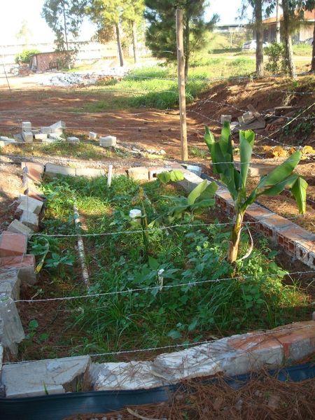
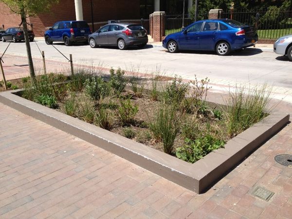
In recent decades, low impact development (LID) practices have started to emerge as BMPs. LID “refers to systems and practices that use or mimic natural processes that result in the infiltration, evapotranspiration or use of stormwater in order to protect water quality and associated aquatic habitat” (USEPA, 2018c). LID is a design approach to managing stormwater runoff in urban and suburban environments, both in new developments and retrofitting older developments. Although the term LID was first coined in the U.S., this paradigm is now widely practiced elsewhere (Saraswat et al., 2016; Hager et al., 2019). Specific BMPs used to support LID include wetlands, which rely on both physical (e.g., settling) and biological (e.g., denitrification) processes to remove water quality pollutants, and bioretention cells, which use infiltration through a bioactive media to remove contaminants and decrease peak flows (Figure 4.2.2). Selection of an appropriate BMP requires knowledge of the specific target pollutants requiring treatment, available land and land cost, and stakeholder preferences and capacity for continuing maintenance. LID approaches also consider the broader ecological impacts beyond the reduction of a target pollutant by the BMPs employed, including habitat restoration and carbon/nutrient cycling.

The advent of these strategies to manage stormwater has partially led to the creation of a new subdiscipline of agricultural and biological engineering during the past few decades, known as ecological engineering. Ecological engineering is defined as “the design of sustainable ecosystems that integrate human society with its natural environment for the benefit of both” (Mitsch, 2012). As with any emerging discipline, there is substantial current research codifying ecological engineering design guidelines and quantifying expected outcomes of relevant BMP implementation (Hager et al., 2019).

Figure \(\PageIndex{2}\): Bioretention cells for urban stormwater control in Brazil (top) and the USA (bottom). These cells are designed to temporarily store water, allowing sediments to settle, and using plants for nutrient uptake. Note the use of local native vegetation.

Urban Stormwater Planning

An important aspect of urban planning is effective stormwater control. The selection of appropriate BMPs for each urban setting depends on the specifics of the situation. For example, consider an urban community that is particularly concerned about maintaining a small downstream reservoir for aquatic recreation. Samples from this reservoir must occasionally be tested for levels of fecal coliform bacteria. The presence of fecal coliform indicates that the water has been contaminated with human or other animal fecal material and that it is possible other pathogenic organisms are present. To ensure fecal coliform values are lower than the recommended levels, specific BMPs can be implemented. Implementing source control practices, such as dog waste collection stations, could be part of the solution. In addition, one or more delivery control practices, such as bioretention cells, detention basins, or a wetland basin, would be required to remove fecal coliforms from stormwater flows. The design of these urban features to reduce coliform transport to local streams and the reservoir requires knowledge of local climate, specifically rainfall patterns and some idea of the loading that might be expected, specifically, the number and magnitude of sources of coliforms. To evaluate which BMP is most appropriate and to obtain design guidelines, a tool such as the International Stormwater BMP Database (Clary et al., 2017) can be used. The database includes data and statistical analyses from over 700 BMP studies, performance analysis results, and other information (International Stormwater BMP Database, 2020). Interpretation of the results of the statistical analysis have to consider issues such as whether the magnitude of the average decrease or the reliability of the BMP is most important, whether the BMP might actually export bacteria, how location specific the data might be, and how useful a particular BMP might be for related pollutants, in this case for something like E. coli. Ultimately size and cost calculations need to be used to select a specific design.

Examples

Example \(\PageIndex{1}\)

Example 1: Quantifying ecosystem services

Problem:

Presently in the U.S. Midwest there is concern that the use of fertilizer on agricultural lands to maximize crop production may result in downstream concentrations of nitrate that render the water more difficult and costly to treat for human consumption. The current maximum permissible concentration of nitrate in drinking water is 10 mg L⁻¹. Assume that the average nitrate concentration in a drinking water treatment plant intake is 12.3 mg L⁻¹. The plant must treat and distribute 1.5 × 10⁸ L of water per day to meet consumer demand. Treating water to remove nitrate costs $2 kg⁻¹. What is the minimum cost of nitrate treatment per year?

Solution

The cost of nitrate treatment is expressed in units of $ kg⁻¹ of nitrate. Thus, to determine the total cost, determine the mass of nitrate treated using Equation 4.2.2:

\( \text{mass nitrate in inflow} = \text{mass nitrate treated} + \text{mass nitrate in outflow} \)

In this case, the concentration of nitrate in the inflow is 12.3 mg L⁻¹. The concentration of nitrate in the outflow should not exceed 10 mg L⁻¹. The difference can be used to estimate the minimum amount of nitrate that must be treated:

\( \text{mass nitrate treated} = \text{(concentration in inflow - concentration in outflow)} \times \text{volume} \)

\( = (12.3\ mg L^{-1} - 10.0\ mg L^{-1} )\times 1.5 \times 10^{8}\ L \text{ day}^{-1} \)

\( = 3.45 \times 10^{8}\ mg \text{ day}^{-1} \times (1\ kg / 10^{6} \ mg) = 345 \text{ kg day}^{-1} \)

The annual cost of treatment can then be calculated as:

\( $2 \text{ kg}^{-1} \times 345 \text{ kg day}^{-1} \times 365 \text{ days year}^{-1} = $251,850 \)

This calculation provides no contingency for inefficiency in the plant. If a safety margin of 1 mg L⁻¹ were included, the outflow concentration would be 9 mg L⁻¹, and the calculation would be:

\( \text{mass nitrate treated} = (12.3 \text{ mg L}^{-1}-9.0 \text{ mg L}^{-1}) \times 1.5 \times 10^{8} \text{ L day}^{-1} \)

\( = 4.95 \times 10^{8} \text{ mg day}^{-1} \times (1 \text{ kg}/10^{6} \text{ mg}) = 495 \text{ kg day}^{-1} \)

and

\( = $2 \text{ kg}^{-1} \times 495 \text{ kg day}^{-1} \times 365 \text{ days year}^{-1} = $361,350 \)

A cost benefit analysis would have to be used to decide whether it was worth paying $109,500 per year for what might be seen as greater certainty that outflow water quality would be better than the permissible limit.

Example \(\PageIndex{2}\)

Example 2: Calculating a TMDL

Problem:

You are a water quality manager tasked with ensuring that a stream within a small, rapidly urbanizing watershed remains in compliance with applicable state standards. At present, water quality monitoring indicates that nitrate-nitrogen (NO₃-N) levels (mg 100 mL⁻¹) in grab samples are just below the state standard. Knowing that future development will likely increase nutrient discharges, you decide to calculate a current TMDL value for future reference based on a current inventory of loadings to the stream. An inventory of local NPDES permits provides the loadings in Table 4.2.1; water quality models estimate that nonpoint sources contribute roughly 2.3 × 10⁹ g month⁻¹ of NO₃-N. Prior experience indicates that the margin of safety should be equivalent to 35% of total current nonpoint and point source loadings in order to account for errors, growth, and missing data. What TMDL value (in Mg day⁻¹) do you report for this stream under the current conditions?

Table \(\PageIndex{1}\): Average daily discharge and NPDES permitted loading from local point sources.

Source	Average Daily Discharge, L day^−1	Permitted Loading (per day)
Wastewater treatment plant	6.4 × 10^6	5.6 × 10^6 E. coli; 0.7 Mg NO3-N
Mid-sized concentrated animal feeding operation (CAFO)	1.0 × 10^4	4.4 × 10^5 E. coli; 0.2 Mg sediment
City storm sewer 1	5.3 × 10^5	10.4 Mg sediment
City storm sewer 2	0.13 × 10^5	3.2 × 10^7 Mg NO3-N

Solution

Calculate the TMDL using Equation 4.2.1; specifically, sum the point (PS) and nonpoint (NPS) source loads of NO₃-N and add a margin of safety (MOS):

\( TMDL = PS+NPS+MOS \)

Point sources of NO₃-N, based on the inventory of local NPDES permits, are a wastewater treatment plant and city storm sewer #2. The total PS loadings per day are:

\( PS = 0.7 Mg\ + 3.2 \times 10^{7} Mg = 3.2 \times 10^{7} Mg\ NO_{3}-N \)

The loading from the wastewater treatment plant is negligible compared to that of the city storm sewer.

Nonpoint sources of NO₃-N are 2.3 × 10⁹ g month⁻¹. Assuming 30 days per month yields the NPS loading per day:

\( NPS = 2.3 \times 10^{9} \text{ g month}^{-1} / (30 \text{ days month}^{-1}) = 77\ Mg\ NO_{3}-N \)

Since the specified margin of safety is 35% of the total PS and NPS loadings, the TMDL is:

\( TMDL = PS+NPS+0.35 (PS+NPS)=1.35\times (PS +NPS)=1.35 \times [(3.2 \times 10^{7})+ 77] \)

\( =4.32 \times 10^{7}\ Mg\ NO_{3}-N \text{ day}^{-1} \)

Example \(\PageIndex{3}\)

Example 3: Nutrient management to meet crop needs

Problem:

You are advising a producer who is managing 30.3 ha in continuous cultivation for corn (maize; Zea mays) silage. You have determined from agronomic advice that for the soil type and cultivar the crop needs 326 kg ha⁻¹ of nitrogen after initial planting. An adjacent dairy has a slurry (mixture of manure and milking parlor wastewater) that could be used as a source of nitrogen. Laboratory analyses indicate that the slurry contains 15.6 kg available nitrogen per 1000 L of slurry.

1. (a) How much slurry would be required to completely fertilize the field to meet crop needs?
2. (b) Assuming the available slurry spreader can spread no less than 47,000 L ha⁻¹, what is the minimum quantity of slurry that can be applied?
3. (c) Is the application of slurry to the field likely to cause pollution?

Solution

1. (a) To calculate the total amount of slurry needed to provide the needed amount of nitrogen to the cropped area, first, calculate the total amount of nitrogen needed in the field:
2. \( N \text{ needed in the field} = 30.3\text{ ha} \times 326 \text{ kg N ha}^{-1} = 9,877.8 \text{ kg N} \)
3. Then, calculate the amount of slurry needed to provide the needed N, based on the N content of the slurry:
4. \( \text{slurry needed in the field} = 9,877.8 \text{ kg N} \times (1,000\ L/15.6 \text{ kg N}) = 633,192\ L \)
5. (b) The machine can apply a minimum of 47,000 L ha⁻¹. Using the available slurry, the amount of nitrogen that would be applied at this rate is:
6. \( 15.6 \text{ kg N} / 1,000\text{ L} \times47,000 \text{ L ha}^{-1} \times 30.3 \text{ ha} = 22,216 \text{ kg N in the field.} \)
7. (c) As the minimum application rate would result in 22,216 kg N applied to the field, and the crop only needs 9,877.8 kg N, there will be an excess of 12,338.2 kg N applied to the field, so it is likely to cause pollution. The producer could consider several options: dilute the available slurry; find another source of slurry with lower concentration of available nitrogen; or find a slurry spreader with a lower minimum spreading rate.

Example \(\PageIndex{4}\)

Example 4: Calculating theoretical detention basin removals by particle size class

Problem:

Assuming theoretical conditions as described above, what is the surface area of a detention basin required to remove 100% of particulates greater than 0.1 mm in size and with a density of 2.6 g cm⁻³? Given the size of the watershed and typical design storm, the basin will need to be designed to treat 10 × 10⁶ m³ of water over 24 hours.

Solution

Detention basins can be sized to completely remove particles of a minimum size and density by setting the overflow rate equal to the theoretical settling velocity for that design size particle.

Calculate overflow rate, Q_R, as expressed by Equation 4.2.4:

\( Q_{R} = \frac{Q}{W \times L} \) (Equation \(\PageIndex{4}\))

\( Q_{R} = \frac{Q}{W \times L} = \frac{\frac{(10 \times 10^{6}\ m^{3})}{24\ hr(3600\ s\ hr^{-1})}}{W \times L} = \frac{11.57\ m^{3}s^{-1}}{W \times L} \)

Calculate the settling velocity (Equation 4.2.5):

\( V_{s} = \frac{gd^{2}(\rho_{p}-\rho_{w})}{18\mu} \) (Equation \(\PageIndex{5}\))

where V_s = settling velocity (m s⁻¹)

ρ_p = density of particle = 2.6 g cm⁻³ = 2,600 kg m⁻³

ρ_w = density of the fluid (water) = 1,000 kg m⁻³

g = acceleration due to gravity = 9.81 m s⁻²

d = particle diameter = 0.1 mm = 0.0001 m

μ = viscosity of water, 10⁻³ N s m⁻² at 20°C

\( V_{s} = \frac{(9.81 m\ s^{-2})(0.0001\ m)^{2}(2,600\ kg\ m^{-3} - 1,000\ kg\ m^{-3})}{18(10^{-3}\ N\ s\ m^{-2})} = 0.00872\ m\ s^{-1} \)

Set overflow rate equal to settling velocity and solve for the required surface area, or W × L, of the detention basin:

\( \frac{11.57\ m^{3}s^{-1}}{W \times L} = 0.00872\ m\ s^{-1} \)

\( W \times L = \frac{11.57\ m^{3}s^{-1}}{0.00872\ m\ s^{-1}} = 1,327\ m^{2} \)

The required surface area of the detention basin is 1,327 m².

Image Credits

Figure 1. Krometis, Leigh-Anne. H. (CC By 4.0). (2020). Theoretical stormwater basin dimensions.

Figure 2. Krometis, Leigh-Anne. H. (CC By 4.0). (2020). Bioretention cells for urban stormwater control in Brazil (top) and the USA (bottom). These cells are designed to temporarily store water, allowing sediments to settle, and using plants for nutrient uptake. Note the use of local native vegetation.

References

APHA. (2013). Improving health and wellness through access to nature. APHA Policy Statement 20137. American Public Health Association. Retrieved from https://www.apha.org/policies-and-advocacy/public-health-policy-statements/policy-database/2014/07/08/09/18/improving-health-and-wellness-through-access-to-nature

ASABE (2020). About the profession. https://asabe.org/About-Us/About-the-Profession

Characklis, G. W., Dilts, M. J., Simmons, III, O. D., Likirduplos, C. A., Krometis, L. A., & Sobsey, M. D. (2005). Microbial partitioning to settleable solids in stormwater. Water Res.39(9), 1773-1782.

Chesapeake Stormwater Network. (2019). Chesapeake Stormwater Network’s urban nutrient management guidelines. Retrieved from https://chesapeakestormwater.net/bmp-resources/urban-nutrient-management/

Clary, J., Strecker, E., Leisenring, M., & Jones, J. (2017). International stormwater BMP database: New tools for a long-term resource. Proc. Water Environment Federation WEFTEC 2017, Session 210–219, pp. 737-746.

EEA. (2019). European Environment Agency. Retrieved from https://www.eea.europa.eu/archived/archived-content-water-topic/wise-help-centre/glossary-definitions/pollution

Freedman, P. L., Nemura, A. D., & Dilks, D. W. (2004). Viewing total maximum daily loads as a process, not a singular value: Adaptive watershed management. J. Environ. Eng., 130, 695-702. https://doi.org/10.1061/(ASCE)0733-9372(2004)130:6(695)

Govenor, H., Krometis, L., & Hession, W. C. (2017). Invertebrate-based water quality impairments and associated stressors identified through the US Clean Water Act. Environ. Manag. 60(4), 598-614.

Hager, J., Hu, G., Hewage, K., & Sadiq, R. (2019). Performance of low-impact development best management practices: A critical review. Environ. Rev., 27(1), 17-42. https://doi.org/10.1007/s00267-017-0907-3.

Hartig, T., Mitchell, R., de Vries, S., & Frumkin, H. (2014). Nature and public health. Ann. Rev. Public Health, 35: 207-228. https://doi.org/10.13140/RG.2.2.15647.61600.

Herngren, L., Goonetilleke, A., & Ayoko, G. A. (2005). Understanding heavy metal and suspended solids relationships in urban stormwater using simulated rainfall. J. Environ. Manag., 76(2), 149-158. https://doi.org/10.1016/j.jenvman.2005.01.013.

Hooke, R. L. (1994). On the efficacy of humans as geomorphic agents. GSA Today 4. Retrieved from https://www.geosociety.org/gsatoday/archive/4/9/pdf/i1052-5173-4-9-sci.pdf.

Hooke, R. L. (2000). On the history of human as geomorphic agent. Geol., 28, 843-846.

International Stormwater BMP Database (2020). http://www.bmpdatabase.org/.

Keeler, B. L., Polasky, S., Brauman, K. A., Johnson, K. A., Finlay, J. C., O’Neill, A., . . . Dalzell, B. (2012). Linking water quality and well-being for improved assessment and valuation of ecosystem services. Proc. Natl. Acad. Sci. USA 109: 18619-18624. http://doi.org/10.1073/pnas.1215991109.

Keller, A. A., & Cavallaro, L. (2008). Assessing the US Clean Water Act 303(d) listing process for determining impairment of a waterbody. J. Environ. Manag., 86, 699-711. http://doi.org/10.1016/j.jenvman.2006.12.013.

MEA. (2005). Ecosystems and human well-being: Biodiversity synthesis. Millennium Ecosystem Assessment. Washington, DC: World Resources Institute. Retrieved from https://www.millenniumassessment.org/documents/document.354.aspx.pdf.

Mitsch, W. 2012. What is ecological engineering? Ecol. Eng., 45, 5-12. https://doi.org/10.1016/j.ecoleng.2012.04.013.

Novotny, V. (2003). Water quality: Diffuse pollution and watershed management. New York, NY: J. Wiley & Sons.

NRC. (2009). Urban stormwater management in the United States. National Research Council. Washington, DC: The National Academies Press. https://doi.org/10.17226/12465.

Raudsepp-Hearne, C., Peterson, G. D., Tengö, M., Bennett, E. M., Holland, T., Benessaiah, K., . . . Pfeifer, L. (2010). Untangling the environmentalist’s paradox: Why is human well-being increasing as ecosystem services degrade? BioSci. 60, 576-589. https://doi.org/10.1525/bio.2010.60.8.4.

Sandifer, P. A., Sutton-Grier, A. E., & Ward, B. P. (2015). Exploring connections among nature, biodiversity, ecosystem services, and human health and well-being: Opportunities to enhance health and biodiversity conservation. Ecosyst. Services 12, 1-15. https://doi.org/10.1016/j.ecoser.2014.12.007.

Saraswat, C., Kumar, P., & Mishra, B. (2016). Assessment of stormwater runoff management practices and governance under climate change and urbanization: An analysis of Bangkok, Hanoi and Tokyo. Environ. Sci. Policy 64, 101-117. https://doi.org/10.1016/j.envsci.2016.06.018.

Sims, J. T., Simard, R. R., & Joern, B. C. (1998). Phosphorus loss in agricultural drainage: Historical perspective and current research. J. Environ. Qual., 27(2), 277-293. doi.org/10.2134/jeq1998.00472425002700020006x.

Tilman, D., Cassman, K. G., Matson, P. A., Naylor, R., & Polasky, S. (2002). Agricultural sustainability and intensive production practices. Nature 418, 671-677. https://doi.org/10.1038/nature01014.

UNFAO. (2019). United Nations Food and Agriculture Organization Aquastat database. Retrieved from http://www.fao.org/nr/water/aquastat/water_use/index.stm.

USEPA. (2018a.) Section 404 of the Clean Water Act. U.S. Environmental Protection Agency. Retrieved from https://www.epa.gov/cwa-404/clean-water-act-section-502-general-definitions.

USEPA. (2018b). Terms and acronyms. U.S. Environmental Protection Agency. Retrieved from https://iaspub.epa.gov/sor_internet/registry/termreg/searchandretrieve/termsandacronyms/search.do.

USEPA. (2018c). Urban runoff: Low impact development. U.S. Environmental Protection Agency. Retrieved from https://www.epa.gov/nps/urban-runoff-low-impact-development.

USEPA. (2019). US EPA’s national summary webpage on water quality impairments and TMDL development. U.S. Environmental Protection Agency. Retrieved from https://ofmpub.epa.gov/waters10/attains_index.home.

USFDA. (2018). Food Safety Modernization Act. U.S. Food and Drug Administration. Retrieved from https://www.fda.gov/food/guidanceregulation/fsma/.

USGS. (2018). Water use in the United States. U.S. Geological Survey. Retrieved from https://water.usgs.gov/watuse/.

Vaze, J., & Chiew, F. H. S. (2004). Nutrient loads associated with different sediment sizes in urban stormwater and surface pollutants. J. Environ. Eng., 130(4), 391-396. https://doi.org/10.1061/(ASCE)0733-9372(2004)130:4(391).

Withers, P., Neal, C., Jarvie, H., & Doody, D. (2014). Agriculture and eutrophication: Where do we go from here? Sustainability 6(9), 5853-5875. https://doi.org/10.3390/su6095853.

World Bank. (2017). Globally, 70% of freshwater is used for agriculture. Retrieved from https://blogs.worldbank.org/opendata/chart-globally-70-freshwater-used-agriculture.

Zgheib, S., Moilleron, R., Saad, M., & Chebbo, G. (2011). Partition of pollution between dissolved and particulate phases: What about emerging substances in urban stormwater cathments? Water Res., 45(2), 913-925. http://doi.org/10.1016/j.watres.2010.09.032.