6.1: Freezing of Food

M. Elena Castell-Perez

Department of Biological and Agricultural Engineering

Texas A&M University, College Station, TX, USA

List of Key Terms

Sensible heat	Freezing point	Cooling load
Specific heat	Conduction	Freezing rate and time
Latent heat	Convection	Freeze drying

Variables for the Chapter

• λ = latent heat of fusion
• ρ = density
• a = thickness
• A = surface area
• C_p = specific heat (also called specific heat capacity)
• h = convective heat transfer coefficient
• k = thermal conductivity
• L = length
• m = mass
• m_A = mass of water in food, or moisture content
• ṁ_p = mass flow rate of product
• M = mass or molecular weight
• M_A = molecular weight of water (18 g/mol)
• M_s = mass of solute in product
• M_s = relative molecular mass of soluble solids in food
• M_S = molecular weight of solute
• M_water = amount of water in product or water content
• P and R = parameters determined by the shape of the food being frozen
• Q_conduction = heat energy transferred through a solid by conduction
• Q_convection = heat energy transferred to a colder moving liquid from the warmer surface of a solid by convection
• Q_L = heat energy removed to freeze the product at its freezing point; also known as latent heat energy
• \(\dot{Q}_{p}\) = rate of heat removed from the food, or cooling load
• Q_p = heat energy removed to freeze the product to the target temperature
• Q_S = sensible heat to change temperature of a food
• R and P = parameters determined by the shape of the food being frozen
• R = universal gas constant (8.314 kJ/kmol)
• t_f = freezing time
• T = temperature
• T_a = freezing medium temperature; ambient temperature
• T_f = freezing point temperature of the food
• x = thickness of packaging material
• ∆x = thickness of the food
• X_i = mass fraction of component i (example: for water, X_water or X_w)

Introduction

Freezing is one of the oldest and more common unit operations that apply heat and mass transfer principles to food. Engineers must know these principles to analyze and design a suitable freezing process and to select proper equipment by establishing system capacity requirements.

Freezing is a common process for long-term preservation of foods. The fundamental principle is the crystallization of most of the water—and some of the solutes—into ice by reducing the temperature of the food to −18°±3°C or lower (a standard commercial freezing target temperature) using the concepts of sensible and latent heat. These principles also apply to freezing of other types of materials that contain water.

If done properly, freezing is the best way to preserve foods without adding preservatives. Freezing aids preservation by reducing the rate of physical, chemical, biochemical, and microbiological reactions in the food. The liquid water-to-ice phase change reduces the availability of the water in the food to participate in any of these reactions. Therefore, a frozen food is more stable and can maintain its quality attributes throughout transportation and storage.

Freezing is commonly used to extend the shelf life of a wide variety of foods, such as fruits and vegetables, meats, fish, dairy, and prepared foods (e.g., ice cream, microwavable meals, pizzas) (George, 1993; James and James, 2014). The great demand for frozen food creates the need for proper knowledge of the mechanics of freezing and material thermophysical properties (Filip et al., 2010).

Outcomes

After reading this chapter, you will be able to:

• • Describe the engineering principles of freezing of foods
• • Describe how food product properties, such as freezing point temperature, size, shape, and composition, as well as packaging, affect the freezing process
• • Describe how process factors, such as freezing medium temperature and convective heat transfer coefficient, affect the freezing process
• • Calculate values of food properties and other factors required to design a freezing process
• • Calculate freezing times
• • Select a freezer for a specific application

Concepts

Process of Freezing

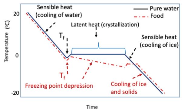
Freezing is a physical process by which the temperature of a material is reduced below its freezing point temperature. Two heat energy principles are involved: sensible heat and latent heat. When the material is at a temperature above its freezing point, first the sensible heat is removed until the material reaches its freezing point; second, the latent heat of crystallization (fusion) is removed, and finally, more sensible heat is removed until the material reaches the target temperature below its freezing point.

Sensible heat is the amount of heat energy that must be added or removed from a specific mass of material to change its temperature to a target value. It is referred to as “sensible” because one can usually sense the temperature surrounding the material during a heating or cooling process. Latent heat is the amount of energy that must be removed in order to change the phase of water in the material. During the phase change, there is no change in the temperature of the material because all the energy is used in the phase change. In the case of freezing, this is the latent heat of fusion. Heat is given off as the product crystallizes at constant temperature.

The comparable term for boiling is the latent heat of vaporization.

For pure water, the latent heat of fusion is a constant with a value of ~334 kJ per kg of water. For food products, the latent heat of fusion can be estimated as

\[ \lambda = M_{water} \times \lambda_{w} \]

where λ = latent heat of fusion of food product (kJ/kg)

M_water = amount of water in product, or water content (decimal)

λ_w = latent heat of fusion of pure water (~334 kJ/kg)

The sensible and latent heat energy in the freezing of foods are quantified by Equations 5.2.2-5.2.9. Table 6.1.1 presents values of the latent heat of several foods with specific moisture contents.

Sensible Heat and Specific Heat

The sensible heat to change the temperature of a food is related to the specific heat of the food, its mass, and its temperature:

\[ Q_{s} = mC_{p}(T_{2}-T_{1}) \]

where Q_S = sensible heat to change temperature of a food (kJ)

m = mass of the food (kg)

C_p = specific heat of the food (kJ/kg°C or kJ/kgK)

T₁ = initial temperature of food (°C)

T₂ = final temperature of food (°C)

The specific heat (also called specific heat capacity), C_p, of liquid water (above freezing) is 4.186 kJ/kg°C or 1 calorie/g°C. In foods, specific heat is a property that changes with the food’s water (moisture) content. Usually, the higher the moisture or water content, the larger the value of C_p, and vice versa. As the water in the food reaches its freezing point temperature, the water begins to crystallize and turn into ice. When almost all of the water is frozen, the specific heat of the food decreases by about half (C_p of ice = 2.108 kJ/kg°C). Therefore, one must be careful when using Equation 6.1.2 to use the correct value of C_p (above or below freezing; see Example 6.1.1 and Equations 6.1.5-6.1.7).

Values of C_p of a wide range of foods at a particular moisture content, above and below freezing, are available (Mohsening, 1980; Choi and Okos, 1986; ASHRAE, 2018; The Engineering Toolbox, 2019; see Table 6.1.1 for some examples). When values of C_p or λ of the target foods are unavailable, they can be determined using several methods, ranging from standard calorimetry to differential scanning, ultrasound, and electrical methods (Mohsenin, 1980; Chen, 1985; Klinbun and Rattanadecho, 2017).

The subscript “p” stands for “constant pressure,” which is the method used to measure the specific heat of solids and liquids. For gases, C_v, or specific heat at constant volume, is used.

When these properties cannot be measured (e.g., because the sample is too small or heterogeneous, or equipment is unavailable), a wide range of models have been developed to predict the properties of food and agricultural materials as a function of time and composition. For instance, if detailed product composition data are not available, Equation 6.1.3 can be used to approximate C_p for temperatures above freezing:

Table \(\PageIndex{1}\): Specific heat (C_p) and latent heat of fusion (λ) of selected foods estimated based on composition (ASHRAE, 2018).

Food	Moisture Content (%)	Cp Above Freezing (kJ/kg°C)	Cp Below Freezing (kJ/kg°C)	λ (kJ/kg)	Tf Initial Freezing Temperature (°C)[a]
Carrots	87.79	3.92	2.00	293	−1.39
Green peas	78.86	3.75	1.98	263	−0.61
Honeydew melon	89.66	3.92	1.86	299	−0.89
Strawberries	91.57	4.00	1.84	306	−0.78
Cod (whole)	81.22	3.78	2.14	271	−2.22
Chicken	65.99	4.34	3.62	220	−2.78

[a] Temperature at which water in food begins to freeze; freezing point temperature.

C_p,unfrozen = C_pwX_w + C_psX_s (3)

where C_pw = specific heat of the water component (kJ/kg°C)

X_w = mass fraction of the water component (decimal)

C_ps = specific heat of the solids component (kJ/kg°C)

X_s = mass fraction of the solids component (decimal)

As a material balance, X_w = 1 – X_s. This method approximates the food as a binary system composed of only water and solids. When the main solids component is known, the C_p of the solids (C_ps) can be estimated from published data (e.g., Table 6.1.2). For instance, if the food is mostly water and carbohydrates (e.g., a fruit), C_ps can be approximated as 1.5488 kJ/kgK (from Table 6.1.2). If the target food is composed mostly of protein, then C_ps can be approximated as 2.0082 kJ/kg°C.

Table \(\PageIndex{2}\): Specific heat, C_p, of food components for −40°C to 150°C.

Food Component	Specific Heat (kJ/kg°C)
Protein
Fat
Carbohydrate
Fiber
Ash

From Choi and Okos, 1986; ASHRAE, 2018. T in °C. An extensive database on food products composition is available in USDA (2019).

The specific heat of the food above its freezing point can be calculated based on its composition and the mass average specific heats of the different components as:

\[ C_{p} = \sum^{n}_{i=1} X_{i}C_{pi} \]

where X_i = mass fraction of component i (decimal, not percentage). For example, for water, X_water = M_water /M where M = total mass of product

i = component (water, protein, fat, carbohydrate, fiber, ash)

C_pi = specific heat of component i estimated at a particular temperature value (kJ/kgK) (from Table 6.1.2)

In the case of water, separate equations are available for liquid water at temperatures below (Equation 6.1.5) and above (Equation 6.1.6) freezing, while one equation applies for ice at temperatures below freezing (Equation 6.1.7) (Choi and Okos, 1986):

For water −40°C to 0°C:

\[ C_{p} = 4.1289-5.3062\times10^{-3}T+9.9516\times 10^{-4} T^{2} \]

For water 0°C to 150°C:

\[ C_{p} = 4.1289-9.0864\times10^{-5}T+5.4731\times 10^{-6} T^{2} \]

For ice −40°C to 0°C:

\[ C_{p} = 2.0623+6.0769\times10^{-3} \]

Many predictive models have been developed for the calculation of specific heat of various food products. Some examples are presented in Table 6.1.3. An excellent description of these and other predictive models is presented in Mohsenin (1980).

Table \(\PageIndex{3}\): Examples of predictive models for calculation of specific heat of foods.

Model, Source	Equation (Cp in kJ/kgK)
Siebel (1892), above freezing[a]	Cp = 0.837 + 3.348Xw
Siebel (1892), below freezing	Cp = 0.837 + 1.256Xw
Chen (1985), above freezing[b]	Cp = 4.19 – 2.30 Xs – 0.628Xs^3
Chen (1985), below freezing[c]	Cp = 1.55 + 1.26 Xs + Xs [R T0^2/MsT^2]
Choi and Okos (1986)	Cp = 4.180Xw + 1.711Xprotein + 1.928Xfat + 1.547Xcarbohydrates + 0.908Xash

[a] X_w = moisture content, decimal; [b] X_s = mass fraction of solids, decimal; [c] R = universal gas constant, 8.314 kJ/kmol K; T₀ = freezing point temperature of water, K; M_s = relative molecular mass of soluble solids in food; T = temperature, K.

Several models, such as a modified version of the model by Chen (1985), are available for simple calculation of the specific heat of a frozen food:

\[ C_{p,frozen} = 1.55+1.26X_{s}+\frac{(X_{w0}-X_{b})\lambda_{w}T_{f}}{T^{2}} \]

where C_p,frozen = apparent specific heat of frozen food (kJ/kgK)

X_s = mass fraction of solids (decimal)

X_w0 = mass fraction of water in the unfrozen food (decimal)

X_b = bound water (decimal); this parameter can be approximated with great accuracy as X_b ~ 0.4X_p (Schwartzberg, 1976) with X_p = mass fraction of protein (decimal)

λ_w = latent heat of fusion of water (~334 kJ/kg)

T_f = freezing point of water = 0.01°C (can be approximated to 0.00°C)

T = food temperature (°C)

Latent Heat

The latent heat of a food product is:

\[ Q_{L}=m\lambda \]

where Q_L = heat energy removed to freeze the product at its freezing point; also known as latent heat energy (kJ)

m = mass of product (kg)

λ = latent heat of fusion of product (kJ/kg)

For water, λ is approximated as 334 kJ/kg. Latent heat values for many food materials are also available (ASHRAE, 2018; Table 6.1.1).

Freezing Point Temperature and Freezing Point Depression

When designing cooling or freezing processes, the heat energy types (Q_S and Q_L) have a negative sign (heat energy is released from the system). When designing heating or thawing processes, these quantities are positive (heat energy is added to the system).

The freezing point temperature, or initial freezing point, of a food product is defined as the temperature at which ice crystals begin to form. Knowledge of this property of foods is essential for proper design of frozen storage and freezing processes because it affects the amount of energy required to reduce the food’s temperature to a specific value below freezing.

Although most foods contain water that turns into ice during freezing, the initial freezing point of most foods ranges from −0.5°C to −2.2°C (Pham, 1987; ASHRAE, 2018); values given in tables are usually average freezing temperatures. Foods freeze at temperatures lower than the freezing point of pure water (which is 0.01°C although most calculations assume 0.0°C) because the water in the foods is not pure water and, when removing heat energy from the food, the freezing point is depressed (lowered) due to the increase in solute concentration in the ice-water sections of the material. Therefore, the food will begin to freeze at temperatures lower than 0 to 0.01°C (Table 6.1.1). This is called the freezing point depression (Figure 6.1.1).

Figure \(\PageIndex{1}\): Freezing curves for pure water and a food product illustrating the concept of freezing point depression (latent heat is released over a range of temperatures when freezing foods versus a constant value for pure water).

In general, 1 g-mol of soluble matter will decrease the freezing point of the product by approximately 1°C (Singh and Heldman, 2013). Consequently, the engineer should estimate the freezing point of the specific product and not assume that the food product will freeze at 0°C.

Some foods with exceptionally low freezing points are dates (−15.7°C), salted yolk (−17.2°C), and cheeses (−16.3 to −1.2°C).

Unfrozen or Bound Water

Water that is bound to the solids in food cannot be frozen. The percent of unfrozen (bound) water at −40°C, a temperature at which most of the water is frozen, ranges from 3% to 46%. This quantity is necessary to determine the heat content of a food (i.e., enthalpy) when exposed to temperatures that cause a phase change; in other words, its latent heat of fusion, λ.

A freezing point depression equation allows for prediction of the relationship between the unfrozen water fraction within the food (X_A) and temperature in a binary solution (i.e., water and solids mixture) over the range from −40°C to 40°C (Heldman, 1974; Chen, 1985; Pham, 1987):

\[ lnX_{A}=\frac{\lambda}{R}(\frac{1}{T_{0}}-\frac{1}{T_{f}}) \]

where X_A = molar fraction of liquid (water) in product A (decimal). (The molar fraction is the number of moles of the liquid divided by the total number of moles of the mixture.)

λ = molar latent heat of fusion of water (6,003 J/mol)

R = universal gas constant (8.314 J/mol K)

T₀ = freezing point of pure water (K)

T_f = freezing point of food (K)

X_A is calculated as

\[ X_{A} = \frac{\frac{m_{A}}{M_{A}}}{\frac{m_{A}}{M_{A}}+\frac{m_{s}}{M_{s}}} \]

where m_A = mass of water in food or moisture content (decimal)

M_A = molecular weight of water (18 g/mol)

M_s = mass of solute in product (decimal)

M_S = molecular weight of solute (g/mol)

Physics of Freezing: Heat Transfer Modes

During freezing of a material, heat is removed within the food by conduction and at its surface by convection, radiation, and evaporation. In practice, these four modes of heat transfer occur simultaneously but with different levels of significance (James and James, 2014). The contributions to heat transfer by radiation and evaporation are much smaller than for the other modes and, therefore, are assumed negligible (Cleland, 2003).

Heat transfer problems can be defined as steady- or unsteady-state situations. During a steady-state process, the temperature within a system (e.g., the food) only changes with location. Hence, temperature does not change with time at that particular location. This is the equilibrium state of a system. One example would be the temperature inside an oven once it has reached the target heating temperature after the food is placed inside the oven. On the other hand, an unsteady-state process (also known as a transient heat transfer problem) is one in which the temperature within the system (e.g., the food) changes with both time and location (the surface, the center, or any distance within the food). Freezing of a product until its center reaches the target frozen storage temperature is a typical unsteady-state problem while storage of a frozen product is a steady-state situation.

Heat Transfer by Conduction

In general, the rate of heat transfer within the food is dominated by conduction and calculated as

\[ Q_{conduction} = kA \Delta T/\Delta x \]

where Q_conduction = heat energy transferred through a solid by conduction (kJ)

k = thermal conductivity of the food (W/m°C)

A = surface area of the food (m²)

∆T = temperature difference within the food (°C)

∆x = thickness of the food (m)

Equation 6.1.12 is valid for one-dimensional heat transfer through a rectangular object of thickness ∆x under steady-state conditions (i.e., equilibrium). Variations of Equation 6.1.12 have been developed for other geometries and are also available in heat transfer textbooks.

Heat Transfer by Convection

Convection controls the rate of heat transfer between the food and its surroundings and is expressed as

\[ Q_{convection} = hA \Delta T \]

where Q_convection = heat energy transferred to a colder moving liquid (air, water, etc.) from the warmer surface of a solid by convection (kJ) during cooling of a solid food

h = convective heat transfer coefficient (W/m²°C)

A = surface area of the solid food (m²)

∆T = temperature difference between the surface of the solid food and the surrounding medium (air, water) = T_surface – T_medium (°C)

The convective heat transfer coefficient, h, is a function of the type of freezing equipment and not of the type of material being frozen. The greater the value of h, the greater the transfer of heat energy from the food’s surface to the cooling medium and the faster the cooling/freezing process at the surface of the food. Measurement and calculation of h values is a function of many factors (James and James, 2014; Pham, 2014). In the case of freezing, the convective heat transfer coefficient varies with selected air temperature and velocity. Table 6.1.4 shows values of h for different types of equipment commonly used in the food industry.

Table \(\PageIndex{4}\): Values of convective heat transfer coefficient, h, and operating temperature for different types of equipment used in food freezing operations.

Freezing Equipment	h (W/m^2K)	Operating (ambient) Freezing Temperature Ta (°C)
Still air (batch)	5 to 20	−35 to −37
Air blast	10 to 200	−20 to −40
Impingement	50 to 200	−40
Spiral belt	25 to 50	−40
Fluidized bed	90 to 140	−40
Plate	100 to 500	−40
Immersion	100 to 500	−50 to −70
Cryogenic	1,500	−50 to −196

Design Parameters: Cooling Load, Freezing Rate, and Freezing Time

The engineer in charge of selecting a cooler or a freezer for a specific type of food needs to know two parameters: the cooling load and the freezing rate, which is related to freezing time.

Cooling Load

The cooling load, also called refrigeration load requirement, is the amount of heat energy that must be removed from the food or the frozen storage space. Here we assume that the rate of heat removed from the product (amount of heat energy per unit time) accounts for the majority of the refrigeration load requirement and that other refrigeration loads, such as those due to lights, machinery, and people in the refrigerated space can be neglected (James and James, 2014). Therefore, the rate of heat transfer between the food and the surrounding cooling medium at any time can be expressed as:

\[ \dot{Q}_{p} = \dot{m}_{p}Q_{p} \]

where \(\dot{Q}_{p}\) = rate of heat removed from the food, i.e., cooling load (kJ/s or kW)

ṁ_p = mass flow rate of product (kg/s)

Q_p = heat energy in the product (kJ)

The computed cooling load is then used to select the proper motor size to carry out the freezing process.

Freezing Rate

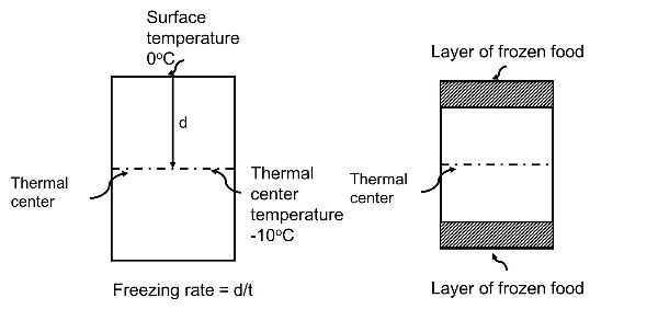
The other critical design parameter is the product freezing rate, which relates to the freezing time. Basically, the freezing rate is the rate of change in temperature during the freezing process. A standard definition of the freezing rate of a food is the ratio between the minimal distance from the product surface to the thermal center of the food (basically the geometric center), d, and the time, t, elapsed between the surface reaching 0°C and the thermal center reaching 10°C colder than the initial freezing point temperature, T_f (IIR, 2006) (Figure 6.1.2). The freezing rate is commonly given as °C/h or in terms of penetration depth measured as cm/h.

Figure \(\PageIndex{2}\): Schematic representation of freezing rate as defined by the International Institute of Refrigeration.

Freezing rate impacts the freezing operation in several ways: food quality, rate of throughput or the amount of food frozen, and equipment and refrigeration costs (Singh and Heldman, 2013). The freezing rate affects the quality of the frozen food because it dictates the amount of water frozen into ice and the size of the ice crystals. Slower rates result in a larger amount of frozen water and larger ice crystals, which may result in undesirable product quality attributes such as a grainy texture in ice cream, ruptured muscle structure in meats and fish, and softer vegetables. Faster freezing produces a larger amount of smaller ice crystals, thus yielding products of superior quality. However, the engineer must take into account the economic viability of selecting a fast freezing process for certain applications (Barbosa-Canovas et al., 2005). Different freezing methods produce different freezing rates.

Freezing Time

Freezing rate and, therefore, freezing time, is the most critical information needed by an engineer to select and design a freezing process because freezing rate (or time) affects product quality, stability and safety, processing requirements, and economic aspects. In other words, the starting point in the design of any freezing system is the calculation of freezing time (Pham, 2014).

Freezing time is defined as the time required to reduce the initial product temperature to some established final temperature at the slowest cooling location, which is also called the thermal center (Singh and Heldman, 2013). The freezing time estimates the residence time of the product in the system and it helps calculate the process throughput (Pham, 2014).

Calculation of freezing time depends on the characteristics of the food being frozen (including composition, homogeneity, size, and shape), the temperature difference between the food and the freezing medium, the insulating effect of the boundary film of air surrounding the material (e.g., the package; this boundary is considered negligible in unpackaged foods), the convective heat transfer coefficient, h, of the system, and the distance that the heat must travel through the food (IRR, 2006).

While there are numerous methods to calculate freezing times, the method of Plank (1913) is presented here. Although this method was developed for freezing of water, its simplicity and applicability to foods make it well-liked by engineers. One modification is presented below.

In Plank’s method, freezing time is calculated as:

\[ t_{f} = \frac{\lambda \rho_{f}}{(T_{f}-T_{a})}(\frac{P_{a}}{h}+\frac{R_{a}^{2}}{k_{f}}) \]

where t_f = freezing time (sec)

λ = latent heat of fusion of the food (kJ/kg); if this value is unknown, it can be estimated using Equation 6.1.1

ρ_f = density of the frozen food (kg/m³) (ASHRAE tables)

T_f = freezing point temperature (°C) (ASHRAE tables or Equation 6.1.10)

T_a = freezing medium temperature (°C) (manufacturer specifications; Table 6.1.4 for examples)

a = the thickness of an infinite slab, the diameter of a sphere or an infinite cylinder, or the smallest dimension of a rectangular brick or cube (m)

P and R = shape factor parameters determined by the shape of the food being frozen (Table 6.1.5).

h = convective heat transfer coefficient (W/m²°C) (Equation 6.1.13 or Table 6.1.4)

k_f = thermal conductivity of the frozen food (W/m°C) (ASHRAE tables)

Table \(\PageIndex{5}\): Shape factors for use in Equations 6.1.15 and 6.1.16 (Lopez-Leiva and Hallstrom, 2003).

Shape	P	R
Infinite plate[a]	1/2	1/8
Infinite cylinder[b]	1/4	1/16
Cylinder[c]	1/6	1/24
Sphere	1/6	1/24
Cube	1/6	1/24

[a] A plate whose length and width are large compared with the thickness

[b] A cylinder with length much larger than the radius (i.e., a very long cylinder)

[c] A cylinder with length equal to its radius

When the dimensions of the food are not infinite or spherical (for example, a brick-shaped product or a box), charts are available to determine the shape factors P and R (Cleland and Earle, 1982).

There are four common assumptions for using Plank’s method to calculate freezing times of food products. Here freezing time is defined as the time to freeze the geometrical center of the product.

• • The first assumption is that freezing starts with all water in the food unfrozen but at its freezing point, T_f, and loss of sensible heat is ignored. In other words, the initial freezing temperature is constant at T_f and the unfrozen center is also at T_f. The food product is not at temperatures above its initial freezing point and the temperature within the food is uniform.
• • The second assumption is that heat transfer takes place sufficiently slowly for steady-state conditions to operate. This means that the food product is at equilibrium conditions and temperature is constant at a specified location (e.g., center or surface of the product). Furthermore, the heat given off is removed by conduction through the inside of the food product and convection at the outside surface, described by combining Equations 6.1.11 and 6.1.12.
• • The third assumption is that the food product is homogeneous and its thermal and physical properties are constant when unfrozen and then change to a different constant value when it is frozen.

  This assumption addresses the fact that thermal conductivity, k, a thermal property of the product that determines its ability to conduct heat energy, is a function of temperature, more importantly below freezing. For instance, a piece of aluminum conducts heat very well and it has a large value of k. On the other hand, plastics are poor heat conductors and have low values of k. Relative to other liquids, water is a good conductor of heat, with a k value of 0.6 W/mK. In the case of foods, k depends on product composition, temperature, and pressure, with water content playing a significant role, similar to specific heat. One distinction is that k is affected by the porosity of the material and the direction of heat (this is called anisotropy). Thus, the higher the moisture content in the food, the closer the k value is to the one for water. Equations to calculate this thermal property as a function of temperature and composition are also provided by Choi and Okos (1986) and ASHRAE (2018). In the case of a frozen food, k_{frozen food} is almost four times larger than the value of unfrozen food since k_ice is approximately four times the value of k_{liquid water} (k_ice = 2.4 W/m°C, k_{liquid water} = 0.6 W/m°C).

  This third assumption also reminds us that the density, ρ, of food materials is affected by temperature (mostly below freezing), moisture content, and porosity. Equations to calculate density as a function of temperature and composition of foods are also provided by Choi and Okos (1986) and ASHRAE (2018). In the case of a frozen food, ρ _{frozen food} is lower than the value of unfrozen food since ρ _ice is lower than ρ _{liquid water} (e.g., ice floats in water).

• • The fourth assumption is that the geometry of the food can be considered as one dimensional, i.e., heat transfers only in the direction of the radius of a cylinder or sphere or through the thickness of a plate and that heat transfer through other directions is negligible.

Despite its simplifying assumptions, Plank’s method gives good results as long as the food’s initial freezing temperature, thermal conductivity, and density of the frozen food are known. Modifications of Equation 6.1.15 provide some improvement but still have limitations (Cleland and Earle, 1982; Pham, 1987). Nevertheless, Plank’s method is widely used for a variety of foods.

One modified version of Plank’s method (Equation 6.1.15) that is commonly used was developed to calculate freezing times of packaged foods (Singh and Heldman, 2013):

\[ t_{f}=\frac{\lambda \rho_{f}}{(T_{f}-T_{a})} [PL(\frac{1}{h} +\frac{x}{k_{2}})+\frac{R_{a}^{2}}{k_{1}}] \]

where L = length of the food (m)

a = thickness of the food (m); assume the food fills the package

x = thickness of packaging material (m)

k₁ = thermal conductivity of packaging material (W/m°C)

k₂ = thermal conductivity of the frozen food (W/m°C)

with other variables as defined in Equation 6.1.15.

The term \(\frac{1}{(\frac{1}{h}+ \frac{x}{k_{2}})}\) is known as the overall convective heat transfer coefficient. It includes both the convective (1/h) and the conductive (x/k₂) resistance to heat transfer through the packaging material.

Applications

Engineers use the concepts described in the previous section to analyze and design freezing processes and to select proper equipment by establishing system capacity requirements. Proper design of a freezing process requires knowledge of food properties including specific heat, thermal conductivity, density, latent heat of fusion, and initial freezing point, as well as the size and shape of the food, its packaging requirements, the cooling load, and the freezing rate and time (Heldman and Singh, 2013). All of these parameters can be calculated using the information described in this chapter.

When the freezing process is not properly designed, it might induce changes in texture and organoleptic (determined using the senses) properties of the foods and loss of shelf life (Singh and Helmand, 2013). Other disadvantages of freezing include the following:

• • product weight losses often range between 4% and 10%;
• • freezing injury of unpackaged foods in slow freezing processes causes cell-wall rupture due to the formation of large ice crystals;
• • frozen products require frozen shipping and storage, which can be expensive;
• • loss of nutrients such as vitamins B and C have been reported; and
• • frozen foods should not be stored for longer than a year to avoid quality losses due to freezer burn (i.e., food surface gets dry and brown).

Because of the potential disadvantages of freezing, proper design of a freezing process also requires the following considerations:

• • the parts of the equipment that will be in contact with the food (e.g., stainless steel) should not impart any flavor or odor to the food;
• • the conditions in the processing plant should be sanitary and allow for easy cleaning;
• • the equipment should be easy to operate;
• • the packaging should be chosen to prevent freezer burn and other quality losses; and
• • the properties of the food that is frozen rapidly may be different from when the food is being frozen slowly.

There is a wide variety of equipment available for freezing of food (Table 6.1.6). The choice of freezing equipment depends upon the rate of freezing required as well as the size, shape, and packaging requirements of the food.

Table \(\PageIndex{6}\): Common types of freezers used in the food industry.

Type of Freezer	Freezing Rate Range
Slow (still-air, cold store)	1°C and 10°C/h (0.2 to 0.5 cm/h)
Quick (air-blast, plate, tunnel)	10°C and 50°C/h (0.5 to 3 cm/h)
Rapid (fluidized-bed, immersion)	Above 50°C/h (5 to 10 cm/h)

Sources: George (1993), Singh (2003), Sudheer and Indira (2007), Pham (2014).

Traditional Freezing Systems

Slow freezers are commonly used for the freezing and storage of frozen foods and are common practice in developing countries (Barbosa-Canovas et al., 2005). Examples of “still” freezers are ice boxes and chest freezers, a batch-type, stationary type of freezer that uses air between −20°C and −30°C. Air is usually circulated by fans (~1.8 m/s). This freezing method is low cost and requires little labor but product quality is low because it may take 3 to 72 h to freeze a 65-kg meat carcass (Pham, 2014).

Quick freezers are more common within the food industry because they are very flexible, easy to operate, and cost-effective for large-throughput operations (George, 1993). Air is forced over the food at 2 to 6 m/s, for an increased rate of heat transfer compared to slow freezers. Blast freezers are examples of this category and are available in batch or continuous mode (in the form of tunnels, spiral, and plate). These quick and blast freezers are relatively economical and provide flexibility to the food processor in terms of type and shape of foods. It takes 10 to 15 minutes to freeze products such as hamburger patties or ice cream (Sudheer and Indira, 2007). Throughput ranges from 350 to 5500 kg/hr.

Rapid freezers are well-suited for individual quick-frozen (IQF) products, such as peas and diced foods, because the very efficient transfer of heat through small-sized products induces the rapid formation of ice throughout the product and, consequently, greater product quality (George, 1993). Fluidized bed freezers are the most common type of freezer used for IQF processes. It usually takes three to four minutes to freeze unpacked peas (Sudheer and Indira, 2007). Throughput ranges from 250 to 3000 kg/hr.

Immersion freezers provide extremely rapid freezing of individual food portions by immersing the product into either a cryogen (a substance that produces very low temperatures, e.g., liquid nitrogen) or a fluid refrigerant with very low freezing temperatures (e.g., carbon dioxide). Immersion freezers also provide uniform temperature distribution throughout the product, which helps maintain product quality. It takes 10 to 15 minutes to freeze many food types (Singh, 2003).

Ultra-rapid freezers (e.g., cryogenic freezers) are suitable for high product throughput rates (over 1500 kg/h), require very little floor space, and are very flexible because they can be used with many types of food products, such as fish fillets, shellfish, pastries, burgers, meat slices, sausages, pizzas, and extruded products (George, 1993). It takes between one-half and one minute to freeze a variety of food items.

Freeze Drying

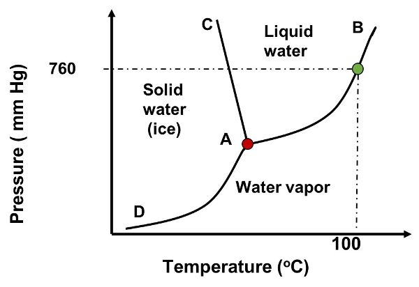
Freeze drying is a specific type of freezing process commonly used in the food industry (McHug, 2018). The process combines drying and freezing operations. In brief, the product is dried (i.e., moisture is removed) using the principle of sublimation of ice to water vapor. Hence, the product is dried at temperature and pressure below the triple point of water. (The triple point is the temperature and pressure at which water exists in equilibrium with its three phases, gas, liquid and solid. At the triple point, T = 0.01°C and P = 611.2 Pa; see Figure 6.1.3.) The A-B line in Figure 6.1.3 represents the saturation (vaporization) line when water transitions from liquid to gas or vice versa; the A-C line represents the line where water transitions from solid to liquid (fusion or melting) or from liquid to solid (solidification or freezing); and the A-D line represents the sublimation line when water transitions from solid to gas directly (as in freeze drying) or when it changes from gas to solid (deposition). Freeze drying is popular for manufacture of rehydrating foods, such as coffee, fruits and vegetables, meat, eggs, and dairy, due to the minimal changes to the products’ physical and chemical properties (Luo and Shu, 2017). This phase change of water occurs at very low pressures.

Figure \(\PageIndex{3}\): Phase diagram of water highlighting the different phases. A (red dot): Triple point of water, 0.01°C and 0.459 mm Hg. A-B line: Saturation (vaporization) line. A-C line: Solidification/fusion line. A-D line: Sublimation/deposition line. The green dot represents the T (100°C) at which water boils at atmospheric pressure (760 mm Hg).

New Freezing Processes

Alternatives to traditional freezing methods are evaluated to make freezing suitable for all types of foods, optimize the amount of energy used and reduce the impact in the environment. Processes such as impingement freezing and hydrofluidization (HF), an immersion type freezer that uses ice slurries, provide higher surface heat-transfer rates with increasing freezing rates, which has tremendous potential to improve the quality of products such as hamburgers or fish fillets (James and James, 2014). These methods use very high velocity air or refrigerant jets that enable very fast freezing of the product. Studies on their applications to foods and other biological materials are in progress. Operating conditions and feasibility of the techniques must be assessed before implementation.

Other promising technologies include high-pressure freezing (also called pressure-shifting freezing) (Otero and Sanz, 2012) and ultrasound-assisted freezing (Delgado and Sun, 2012), which facilitate formation of smaller ice crystals. Magnetic resonance and microwave-assisted freezing, cryofixation, and osmodehydrofreezing are other new freezing technologies. Another trend is “smart freezing” technology, which combines the mechanical aspects of freezing with sensor technologies to track food quality throughout the cold chain. Smart freezing uses computer vision and wireless sensor networks (WSN), real-time diagnosis tools to optimize the process, ultrasonic monitoring of the freezing process, gas sensors to predict crystal size in ice cream, and temperature-tracking sensors to predict freezing times and product quality (Xu et al., 2017).

Examples

Examples 6.1.1 through 6.1.6 show a few of the many options an engineer could consider when selecting the best type of freezing equipment and operational parameters to freeze a food product. Another critical aspect of design of freezing processes for foods is that many of the products are packaged and the packaging material offers resistance to the transfer of heat, thus increasing freezing time (Yanniotis, 2008). Example 6.1.7 illustrates this point.

Example \(\PageIndex{1}\)

Example 1: Calculation of refrigeration requirement to freeze a food product

Problem:

Calculate the refrigeration requirement when freezing 2,000 kg of strawberries (91.6% moisture) from an initial temperature of 20°C to −20°C. The initial freezing point of strawberries is −0.78°C (Table 6.1.1).

Solution

(1) identify the type of heat process(es) involved in this process and set up the energy balance; (2) calculate how much heat energy must be removed from the strawberries to carry out the freezing process; and (3) calculate the refrigeration requirement (in kW) for the freezing process.

The following assumptions are commonly made in this type of calculation:

• • Conservation of mass during the freezing process. Thus, m_strawberries = 2,000 kg remains constant because the fruits do not lose or gain moisture (or the changes in mass are negligible).
• • The freezing point temperature is known.
• • The temperature of the freezing medium (ambient temperature) and storage remains constant (i.e., a steady-state situation).

Step 1 Identify the type of heat processes and set up the energy balance:

• • Sensible, to decrease the temperature of the strawberries from 20°C to just when they begin to crystallize at −0.78°C
• • Latent, to change liquid water in strawberries to ice at −0.78°C
• • Sensible, to further cool the strawberries to −20°C (using Equation 6.1.2)

Thus, for the given freezing process, the heat energy balance is the sum of the three heat processes listed above.

Step 2 Calculate the total amount of energy removed in the freezing process, Q:

Sensible, from 20°C to −0.78°C, using Equation 6.1.2, where Q_s = Q₁:

\( Q_{1}=mC_{p,frozen}(T_{2}-T_{1}) \) (Equation \(\PageIndex{2}\))

where m = 2,000 kg

T₁ = 20°C

T₂ = −0.78°C

C_p of unfrozen strawberries (at 91.6 % moisture) = 4.00 kJ/kg°C (Table 6.1.1). See Example 6.1.2 for calculation of the specific heat of a food product above freezing.

Thus,

Q₁ = (2,000 kg)(4.00 kJ/kg°C)(−0.78 – 20°C) = −166,240 kJ

Note that this value is negative because heat is released from the product.

Latent, using Equation 6.1.9:

\( Q_{2}=m\lambda \text{ at } T = -0.78 ^\circ C \) (Equation \(\PageIndex{9}\))

where m = 2,000 kg

λ = latent heat of fusion of strawberries at given moisture content = 306 kJ/kg (from Table 6.1.1).

Thus,

Q₂ = (2,000 kg)(306 kJ/kg) = −612,000 kJ

Note that this value is negative because heat is being released from the product.

Sensible, to further cool to −20°C, again using Equation 6.1.2:

\( Q_{3}=mC_{p,frozen}(T_{2}-T_{1}) \) (Equation \(\PageIndex{2}\))

where m = 2,000 kg

T₁ = −0.78°C

T₂ = −20°C

C_p of frozen strawberries (at 91.6 % moisture) = 1.84 kJ/kg°C (Table 6.1.1). See Example 6.1.3 for calculation of the specific heat of a frozen food product.

Thus,

Q₃ = (2,000 kg)(1.84 kJ/kg°C)(−20 + 0.78°C) = −70,729.6 kJ

Adding all energy terms:

Q = Q₁ + Q₂ + Q₃ = −166,240 kJ – 612,000 kJ – 70,729.6 kJ

= −848,969.6 kJ = Q_product

The heat energy removed per kg of strawberries:

Q_product per kg of fruit = −848,969.6 kJ/2,000 kg = −424.48 kJ/kg

Thus, 848,969.6 kJ of heat must be removed from the 2,000 kg of strawberries (424.48 kJ/kg) initially held at 20°C to freeze them to the target storage temperature of −20°C.

Step 3 Calculate the refrigeration requirement, or cooling load (in kW), for the freezing process. The cooling load \(\dot{Q}_{p}\) (also called refrigeration requirement) to freeze 2,000 kg/h of strawberries from 20°C to −20°C is calculated with Equation 6.1.14:

\( \dot{Q}_{p} = \dot{m}_{p}Q_{p} \) (Equation \(\PageIndex{14}\))

where ṁ_p = mass flow rate of product (kg/s)

Q_p = heat energy removed to freeze the product to the target temperature = −424.48 kJ/kg

\(\dot{Q}_{p}\) = (2,000 kg/h × −424.48 kJ/kg) /3600 s = −235.82 kJ/s or kW

Note that 1 kJ/s = 1 kilowatt = 1 kW.

Example \(\PageIndex{2}\)

Example 2: Determine the initial freezing point (i.e., temperature at which water in food begins to freeze) and the latent heat of fusion of a food product

Problem:

Determine the initial freezing point and latent heat of fusion of green peas with 79% moisture.

Solution

Solution by use of tables:

From Table 6.1.1, the T_f of green peas at the given moisture content is −0.61°C and the latent heat of fusion λ is 263 kJ/kg.

Solution by calculation:

If tabulated λ values are not available, λ of the product can be estimated using Equation 6.1.1.

\( \lambda = M_{water} \times \lambda_{w} \) (Equation \(\PageIndex{1}\))

λ = (0.79) × (334 kJ/kg) = 263.86 kJ/kg

Example \(\PageIndex{3}\)

Example 3: Estimation of specific heat of a food product based on composition

Sometimes the engineer will not have access to measured or tabulated values of the specific heat of the food product and will have to estimate it in order to calculate cooling loads. This example provides some insight into how to estimate specific heat of a food product.

Problem:

Calculate the specific heat of honeydew melon at 20°C and at −20°C. Composition data for the melon is available as 89.66% water, 0.46% protein, 0.1% fat, 9.18% total carbohydrates (includes fiber), and 0.6% ash (USDA, 2019). Give answers in the SI units of kJ/kgK.

Solution

Use Equations 6.1.5-6.1.7 to account for the effect of product composition and temperature on specific heat. The specific heat of honeydew at T = 20°C is calculated using Equation 6.1.4:

\( C_{p}=\sum^{n}_{i=1}X_{i}C_{pi} \) (Equation \(\PageIndex{4}\))

Thus,

\( C_{p,honeydew}=X_{w}C_{pw}+X_{p}C_{pp}+X_{f}C_{pf}+X_{c}C_{pf}+X_{a}C_{pa} \)

with subscripts w, p, f, c, and a representing water, protein, fat, carbohydrates, and ash, respectively, and C_p in kJ/kg°C.

Step 1 Calculate the C_p of water (C_pw) at 20°C using Equation 6.1.6:

C_p = 4.1289 – 9.0864 × 10⁻⁵ T + 5.4731 × 10⁻⁶T² (6)

Thus,

C_p = 4.1289 – (9.0864 × 10⁻⁵)(20) + (5.4731 × 10⁻⁶)(20)²

C_pw = 4.127 kJ/kg°C

Step 2 Calculate the specific heat of the different components at T = 20°C using the equations given in Table 6.1.2.

Food Component	Cp of Honeydew at T = 20°C (kJ/kgK)
Water	4.127
Protein	2.032
Fat	2.012
Carbohydrate	1.586
Fiber	NA
Ash	1.129

Step 3 Calculate the specific heat of honeydew at 20°C using Equation 6.1.4:

\( C_{p,honeydew}=(0.8966)(4.127)+(0.0046)(2.032)+(0.001)(2.012)+(0.0918)(1.586)+(0.006)(1.129) \)

C_p,honeydew at 20°C = 3.86 kJ/kg°C

Step 4 Calculate the specific heat of honeydew at −20°C using Equation 6.1.8:

\( C_{p,frozen} = 1.55 + 1.26X_{s}+\frac{(X_{w0}-X_{b})L_{0}T_{f}}{T^{2}} \) (Equation \(\PageIndex{8}\))

From the given composition of honeydew:

X_s = mass fraction of solids = 1 – 0.8966 = 0.1034

X_w0 = mass fraction of water in the unfrozen food = 0.8966

X_b = bound water = 0.4X_p = 0.4(0.0046) = 0.00184

T_f = freezing point of food to be frozen = −0.89°C (from Table 6.1.1)

T = food target (or freezing process) temperature = −20°C

Substituting the numbers into Equation 6.1.8:

\( C_{p,frozen} = 1.55 + 1.26X_{s}+\frac{(X_{w0}-X_{b})L_{0}T_{f}}{T^{2}} \) (Equation \(\PageIndex{8}\))

\( C_{p,frozen} = 1.55 + 1.26(0.1034)+\frac{(0.8966-0.00184)(\frac{334 \ kJ}{kg})(-0.89^\circ C)}{(-20^\circ C)^{2}} \)

C_p,frozen = 2.397 kJ/kg°C

The calculated C_p values can then be used to calculate cooling load as shown in Example 6.1.1.

Observations:

• • As expected, the specific heat of the frozen honeydew is lower than the value for the fruit above freezing.
• • When values of the product’s specific heat and initial freezing point are not available from tables, engineers should be able to estimate them using available prediction models and composition data.
• • The C_p of the frozen product was calculated at −20°C, the freezing process temperature. Tabulated values are usually given when the food is fully frozen at a reference temperature of −40°C (ASHRAE, 2018). If we use −40°C in Equation 6.1.8, then

\( C_{p,frozen} = 1.55 + 1.26(0.1034)+\frac{(0.8966-0.00184)(\frac{334 \ kJ}{kg})(-0.89^\circ C)}{(-40^\circ C)^{2}} \)

C_p,frozen = 1.85 kJ/kg°C.

• This value is closer to the tabulated values. While the change in C_p as a function of temperature can be important in research studies, it does not influence the selection of freezing equipment.
• • Many mathematical models are available for prediction of specific heat and other properties of foods (Mohsenin, 1980; Choi and Okos, 1986; ASHRAE, 2018). The engineer must choose the value that is more suitable for the specific application using available composition and temperature data.

Example \(\PageIndex{4}\)

Example 4: Calculation of initial freezing point temperature of a food product

Problem:

Consider the strawberries in Example 6.1.1 and calculate the depression of the initial freezing point of the fruit assuming the main solid present in the strawberries is fructose (a sugar), with molecular weight of 108.16 g/mol.

Solution

Calculation of the initial freezing point temperature requires a series of steps.

Step 1 Collect all necessary data. From Example 6.1.1, strawberries contain 91.6% water (m_A) and the rest is fructose (100 – 91.6 = 8.04% solids = m_s). Other information provided is M_s = M_fructose = 108.16 g/mol, λ = 6,003 J/mol, M_A = 18 g/mol, R = 8.314 J/mol K, and T₀ = 273.15 K.

Step 2 Calculate X_A, the molar fraction of liquid (water) in the strawberries (decimal) using Equation 6.1.11:

\( X_{A} = \frac{\frac{0.916}{18}}{\frac{0.916}{18}+\frac{0.0804}{108.16}} = 0.9922 \)

Step 3 Calculate T_f of strawberries using Equation 6.1.10:

\( nX_{A}=\frac{\lambda}{R}(\frac{1}{T_{0}}-\frac{1}{T_{f}}) \) (Equation \(\PageIndex{10}\))

Rearranged:

\( T_{f} = (\frac{R}{\lambda}lnX_{A}-\frac{1}{T_{0}})^{-1} \)

\( T_{f} = (\frac{8.314\text{ J/mol K}}{6003\text{ J/mol}}ln(0.9922)-\frac{1}{273.15})^{-1} \)

\( T_{f} = 272.34\ K = -0.81^\circ C \)

Observation:

The presence of fructose in the strawberries results in an initial freezing point temperature lower than that for pure water.

Example \(\PageIndex{5}\)

Example 5: Calculation of freezing time of an unpackaged food product

An air-blast freezer is used to freeze cod fillets (81.22% moisture, freezing point temperature = −2.2°C, initial temperature = 5°C, mass of fish = 1 kg). Assume that each cod fillet is an infinite plate with thickness of 6 cm. Freezing process parameters for the air-blast freezer are: freezing medium temperature −20°C, convective heat transfer coefficient, h, of 50 W/m²°C (Table 6.1.4), the density and thermal conductivity of the frozen fish are 992 kg/m³ and 1.9 W/m°C, respectively (ASHRAE, 2018). The target freezing time is less than 2 hours.

Problem:

Calculate the time required to freeze a fish fillet (freezing time, t_f), using Plank’s method (Equation 6.1.15):

\( t_{f}=\frac{\lambda \rho_{f}}{(T_{F}-T_{a})}(\frac{P_{a}}{h}+\frac{R^{2}_{a}}{k_{f}}) \) (Equation \(\PageIndex{15}\))

Solution

Step 1 Determine the required food and process parameters:

λ = latent heat of fusion of cod fillet = 271.27 kJ/kg (from tables, ASHRAE, or calculated using Equation 6.1.1, λ = (0.8122)(334 kJ/kg) = 271.27 kJ/kg = 271.27 × 10³ J/kg)

ρ_f = density of the frozen food, 992 kg/m³ (from ASHRAE, 2018)

T_f = freezing point temperature, −2.2°C (available in ASHRAE, 2018, or calculated using composition and Equations 6.1.10 and 6.1.11)

T_a = freezing medium temperature, −20°C

a = thickness of the plate = 6 cm = 0.06 m

P and R = shape factor parameters, 1/2 and 1/8 (from Table 6.1.6)

h = convective heat transfer coefficient, 50 W/m²°C (given)

k_f = thermal conductivity of the frozen food, 1.9 W/m°C (from ASHRAE)

Step 2 Calculate the freezing time, t_f, from Equation 6.1.15 as:

\( t_{f}=\frac{(271.27\times10^{3}\frac{J}{kg})\frac{992\ kg}{m^{3}}}{[(-2.2)-(20C)]}[\frac{(0.06\ m)}{2(\frac{50\ W}{m^{2}C})}+\frac{(0.06\ m)^{2}}{8(\frac{1.9\ W}{mC})}] \)

t_f = 12,651.35 seconds/3600 = 3.5 h. The freezing time target would not be met.

Reminder:

Plank’s method calculates the time required to remove the latent heat to freeze the fish. It does not take into account the time required to remove the sensible heat from the initial temperature of 5°C to the initial freezing point. This means that use of Equation 6.1.15 might underestimate freezing times.

As shown in Example 6.1.1, Q_S, the sensible heat removed to decrease the temperature of the fish from 5°C to just when it begins to crystallize at −2.2°C is calculated using Equation 6.1.2:

\( Q_{s}=mC_{p}(T_{2}-T_{1}) \) (Equation \(\PageIndex{2}\))

where m = mass of the food = 1 kg

C_p = specific heat of the unfrozen cod (at 81.22 % moisture) = 3.78 kJ/kg°C (from tables, ASHRAE, 2018).

T₁ = 5°C

T₂ = −2.2°C

Thus, Q_S = (1 kg)(3.78 kJ/kg°C)(−2.2 – 5°C) = −27.216 kJ = −27,216 J of heat energy removed per kg of fish. The quantity is negative because heat is released from the product when it is cooled. Also, although not negligible, this amount is much lower than the latent heat removal.

Example \(\PageIndex{6}\)

Example 6: Find ways to decrease freezing time of an unpackaged food product

Problem:

Find a way to decrease freezing time of the cod fillets in Example 6.1.5 to less than 2 hours.

Solution

Evaluate the effect (if any) of some process and product variables on the calculated freezing time, t_f, using Plank’s method and determine which parameters decrease freezing time. Equation 6.1.15:

\( t_{f}=\frac{\lambda \rho_{p}}{(T_{F} - T_{a})}(\frac{P_{a}}{h}+\frac{R_{a}^{2}}{k_{f}}) \) (Equation \(\PageIndex{15}\))

Freezing process variables:

• • Freezing time decreases when freezing medium temperature, T_a, decreases (colder medium):

\( t_{f} \propto \frac{1}{(T_{F}-T_{a})} \)

• • Freezing time decreases when the convective heat transfer coefficient, h, increases (faster removal of heat energy and thus faster freezing process):

\( t_{f} \propto \frac{1}{h} \)

Product variables:

• • Freezing time decreases when the thickness, a, of the product decreases (smaller product):

\( t_{f} \propto (\frac{a}{h}+\frac{a^{2}}{k_{f}}) \)

• • Freezing time decreases when the product shape changes from a plate to a cylinder or a sphere (greater surface area), i.e., P decreases from 1/2 to 1/6 and R decreases from 1/8 to 1/24:

\( t_{f} \propto (\frac{P}{h}+\frac{R}{k_{f}}) \)

• • Freezing time decreases with a lower latent heat of fusion of the food, λ, a lower density of the frozen food, ρ_f, and a higher thermal conductivity of the frozen food, k_f:

\( t_{f} \propto \lambda \rho_{f}(\frac{1}{k_{f}}) \)

• This highlights the need for accurate values for these variables when using this method to calculate freezing times.
• • The effect of the initial freezing point is less significant due to the small range of variability among a wide variety of food products:

\( t_{f} \propto \frac{1}{(T_{f}-T_{a})} \)

Changing freezing process variables. Do the calculation assuming a freezing medium temperature of −40°C (Table 6.1.4) instead of the T_a = −20°C used in Example 6.1.5, while holding everything else constant:

\( t_{f}=\frac{(271.27\times10^{3}\frac{J}{kg})\frac{992\ kg}{m^{3}}}{[(-2.2)-(40C)]}[\frac{(0.06\ m)}{2(\frac{50\ W}{m^{2}C})}+\frac{(0.06\ m)^{2}}{8(\frac{1.9\ W}{mC})}] \)

t_f = 5957.51 seconds ~1.66 h < 2 h. The freezing time target would be met.

This result makes sense because the lower the temperature of the freezing medium (air, in an air-blast freezer), the shorter the freezing time.

Next, consider increasing the convective heat transfer coefficient, h, for the air-blast freezer. Based on Table 6.1.4, this variable can go as high as 200 W/m°C for this type of freezer. While holding everything else constant,

\( t_{f}=\frac{(271.27\times10^{3}\frac{J}{kg})(\frac{992\ kg}{m^{3}})}{[(-2.2)-(20C)]}[\frac{(0.06\ m)}{2(\frac{200\ W}{m^{2}C})}+\frac{(0.06\ m)^{2}}{8(\frac{1.9\ W}{mC})}] \)

t_f = 5848.27 seconds ~ 1.63 h < 2 h. The freezing time target would be met.

This result also makes sense because the faster the freezing rate (due to higher h value), the shorter the freezing time.

Achieving the target freezing time of less than 2 hours would require a change in the freezing process parameters of the air-blast freezer, either the convective heat transfer coefficient h or the operating conditions (the freezing medium temperature, T_a).

Changing product variables. Try changing the thickness, a. Assume the fish is frozen as fillets that are 3 cm thick (half the thickness of the original design). Holding everything else constant except now a = 0.03 m,

\( t_{f}=\frac{(271.27\times10^{3}\frac{J}{kg})(\frac{992\ kg}{m^{3}})}{[(-2.2)-(20C)]}[\frac{(0.03\ m)}{2(\frac{50\ W}{m^{2}C})}+\frac{(0.06\ m)^{2}}{8(\frac{1.9\ W}{mC})}] \)

t_f = 5430.53 seconds = 1.5 h < 2 h. The freezing time target would be met.

In this case, there is no need to change the operating conditions of the air-blast freezer.

Next, change the shape of the product. Fillets can be shaped as infinite (very long) cylinders (P and R = 1/4 and 1/16, respectively; Table 6.1.5) with 6 cm diameter, instead of as long plates. Keeping everything else constant and using the original freezing process parameters:

\( t_{f}=\frac{(271.27\times10^{3}\frac{J}{kg})(\frac{992\ kg}{m^{3}})}{[(-2.2)-(20C)]}[\frac{(0.06\ m)}{4(\frac{50\ W}{m^{2}C})}+\frac{(0.06\ m)^{2}}{16(\frac{1.9\ W}{mC})}] \)

t_f = 6325.68 seconds = 1.76 h < 2 h. The freezing time target would be met.

This result illustrates the significance of product shape on the rate of heat transfer and, consequently, freezing time. In general, a spherical product will freeze faster than one of similar size with the shape of a cylinder or a plate due to its greater surface area.

Example \(\PageIndex{7}\)

Example 7. Calculation of freezing time of a packaged food product

For this example, assume that the cod fish from Example 6.1.5 is packed into a cardboard carton measuring 10 cm × 10 cm × 10 cm. The carton thickness is 1.5 mm and its thermal conductivity is 0.065 W/m°C.

Problem:

Calculate the freezing time using the original freezing process parameters (h = 50 W/m²°C, T_a = −20°C) and determine whether the product can be frozen in 2 to 3 hours. If not, provide recommendations to achieve the desired freezing time.

Solution

Because the food is packaged, use the modified version of Plank (Equation 6.1.16):

\( t_{f} = \frac{\lambda \rho_{f}}{(T_{f}-T_{a})}[PL(\frac{1}{h}+\frac{x}{k_{2}})+\frac{R_{a}^{2}}{k_{1}}] \) (Equation \(\PageIndex{16}\))

Step 1 Collect the information needed from Example 6.1.5. Also,

L = length of the food = 10 cm = 0.1 m

a = 10 cm = 0.1 m

x = thickness of packaging material = 1.5 mm = 0.0015 m

k₂ = thermal conductivity of packaging material = 0.065 W/m°C

k₁ = thermal conductivity of the frozen fish =1.9 W/m°C

Step 2 Calculate the freezing time:

\( t_{f} = \frac{(271.27\times10^{3} \frac{J}{kg})(992 \frac{kg}{m^{3}})}{17.8^\circ C}[\frac{0.1\ m}{6}(\frac{1}{50}+\frac{0.0015}{0.065})+(\frac{(0.1\ m)^{2}}{24(1.9)})] \)

t_f = 14,200.28 seconds = 3.9 h >>>> 2 to 3 h.

The freezing time target would not be met.

The freezing process must be modified. Note that freezing of the fish when packaged in cardboard takes longer than the unpackaged product.

Step 3 Calculate some possible options to reduce the freezing time.

• • Shorten the freezing time by using a higher convective heat transfer coefficient, h, of 100 W/m²°C. Then,

\( t_{f} = \frac{(271.27\times10^{3} \frac{J}{kg})(992 \frac{kg}{m^{3}})}{17.8^\circ C}[\frac{0.1\ m}{6}(\frac{1}{100}+\frac{0.0015}{0.065})+(\frac{(0.1\ m)^{2}}{24(1.9)})] \)

t_f = 11649.6 seconds = 3.23 h.

• The freezing time target would not be met.
• • Shorten the freezing time by using a yet higher h of 200 W/m²°C. Then,

\( t_{f} = \frac{(271.27\times10^{3} \frac{J}{kg})(992 \frac{kg}{m^{3}})}{17.8^\circ C}[\frac{0.1\ m}{6}(\frac{1}{200}+\frac{0.0015}{0.065})+(\frac{(0.1\ m)^{2}}{24(1.9)})] \)

t_f = 10389.8 seconds = 2.9 h.

• The freezing time target would be met.
• • Shorten freezing time by using h = 100 W/m²°C and changing the temperature of the freezing medium, T_a, to −40°C:

\( t_{f} = \frac{(271.27\times10^{3} \frac{J}{kg})(992 \frac{kg}{m^{3}})}{37.88^\circ C}[\frac{0.1\ m}{6}(\frac{1}{200}+\frac{0.0015}{0.065})+(\frac{(0.1\ m)^{2}}{24(1.9)})] \)

t_f = 5485.8 seconds = 1.5 h.

This is closer to the target freezing time for the unpackaged fish.

Freezing time could also be reduced by using a different packaging material. For example, plastics have higher k₂ values than cardboard, decreasing product resistance to heat transfer.

Note that changing the shape of the packaging container to a cylinder would not have an effect on freezing time since P and R are the same as for a cube.

Example \(\PageIndex{8}\)

Example 8. Selection of freezer

The choice of freezer equipment depends on the cost and effect on product quality. Overall, the engineer will need to consider a faster freezing process when dealing with foods packaged in cardboard, compared to unpackaged products or food packaged in plastic.

Problem:

For this example, compare the freezing times for a typical plate freezer to that of a spiral belt freezer.

Solution

Step 1 Calculate the freezing time for the packaged product in Example 6.1.7 using a plate freezer that produces h = 300 W/m²°C at T_a = −40°C:

\( t_{f} = \frac{(271.27\times10^{3} \frac{J}{kg})(992 \frac{kg}{m^{3}})}{37.8^\circ C}[\frac{0.1\ m}{6}(\frac{1}{300}+\frac{0.0015}{0.065})+(\frac{(0.1\ m)^{2}}{24(1.9)})] \)

t_f = 4694.8 seconds = 1.3 h

Step 2 Calculate the freezing time for the packaged product in Example 6.1.7 using a spiral freezer that produces h = 30 W/m²°C at T_a = −40°C:

\( t_{f} = \frac{(271.27\times10^{3} \frac{J}{kg})(992 \frac{kg}{m^{3}})}{37.8^\circ C}[\frac{0.1\ m}{6}(\frac{1}{30}+\frac{0.0015}{0.065})+(\frac{(0.1\ m)^{2}}{24(1.9)})] \)

t_f = 32893.2 seconds = 9 h.

This spiral freezer would not be suitable in terms of freezing time.

Image Credits

Figure 1. Castell-Perez, M. Elena. (CC By 4.0). (2020). Freezing curves for pure water and a food product illustrating the concept of freezing point depression (latent heat is released over a range of temperatures when freezing foods versus a constant value for pure water).

Figure 2. Castell-Perez, M. Elena. (CC By 4.0). (2020). Schematic representation of the International Institute of Refrigeration definition of freezing rate.

Figure 3. Castell-Perez, M. Elena. (CC By 4.0). (2020). Phase diagram of water highlighting the different phases. A (red dot): triple point of water, 0.00098°C and 0.459 mmHg. A-B line: saturation (vaporization) line. B-C line Solidification/fusion line. A-D line: Sublimation line. The green dot represents the T (100°C).

References

ASHRAE. (2018). Thermal properties of foods. In ASHRAE Handbook—Refrigeration (Chapter 19). American Society of Heating, Refrigeration and Air Conditioning. https://www.ashrae.org/.

Note: This source should be available in libraries at universities and colleges with engineering programs. It consists of four volumes with the one on “Refrigeration” being the most relevant to this chapter.

Barbosa-Cánovas, G. V., Altukanar, B., & Mejia-Lorio, D. J. (2005). Freezing of fruits and vegetables. An agri-business alternative to rural and semi-rural areas. FAO Agricultural Services Bulletin 158. Food and Agriculture Organization of the United Nations. http://www.fao.org/docrep/008/y5979e/y5979e00.htm#Contents.

Chen, C. S. (1985) Thermodynamic analysis of the freezing and thawing of foods: Enthalpy and apparent specific heat. J. Food Sci. 50(4), 1158-1162. doi.org/10.1111/j.1365-2621.1985.tb13034.x.

Choi, Y., & Okos, M. R. (1986) Effect of temperature and composition on the thermal properties of foods. In M. Le Maguer and P. Jelen (Eds.), Food Engineering and Process Applications (Vol.1, pp.93-101). Elsevier.

Cleland, A. C., & Earle, R. L. (1982). Freezing time prediction for foods—A simplified procedure. Int. J. Ref. 5(3), 134-140. https://doi.org/10.1016/0140-7007(82)90092-5

Cleland, D. J. (2003). Freezing times calculation. In Encyclopedia of Agricultural, Food, and Biological Engineering (pp. 396-401). Marcel Dekker, Inc.

Delgado, A., & Sun, D. W. (2012) Ultrasound-accelerated freezing. In D. W. Sun (Ed.), Handbook of Frozen Food Processing and Packaging (2nd ed., Chapter 28, pp. 645-666). CRC Press.

Engineering Toolbox. 2019. Specific heat of food and foodstuff. https://www.engineeringtoolbox.com/specific-heat-capacity-food-d_295.html. Accessed 8 July 2019.

Filip, S., Fink, R., & Jevšnik, M. (2010). Influence of food composition on freezing time. Int. J. Sanitary Eng. Res. 4, 4-13.

George, R. M. (1993). Freezing processes used in the food industry. Trends in Food Sci. Technol. 4(5), 134-138. https://doi.org/10.1016/0924-2244(93)90032-6.

Heldman, D. R. (1974). Predicting the relationship between unfrozen water fraction and temperature during food freezing using freezing point depression. Trans. ASAE 17(1), 63-66. https://doi.org/10.13031/2013.36788.

IRR. (2006). Recommendations for the Processing and Handling of Frozen Foods. International Institute of Refrigeration.

James, S. J., & James, C. (2014). Chilling and freezing of foods. In S. Clark, S. Jung, & B. Lamsal (Eds.), Food Processing: Principles and Applications (2nd ed., Chapter 5). Wiley.

Klinbun, W., & Rattanadecho, P. (2017). An investigation of the dielectric and thermal properties of frozen foods over a temperature from −18 to 80°C. Intl. J. Food Properties 20(2), 455-464. https://doi.org/10.1080/10942912.2016.1166129.

Lopez-Leiva, M., & Hallstrom, B. (2003). The original Plank equation and its use in the development of food freezing rate predictions. J. Food Eng. 58(3), 267-275. https://doi.org/10.1016/S0260-8774(02)00385-0.

Luo, N., & Shu, H. (2017). Analysis of energy saving during food freeze drying. Procedia Eng. 205, 3763-3768. https://doi.org/10.1016/j.proeng.2017.10.330.

McHug, T. (2018). Freeze-drying fundamentals. Food Technol. 72(2), 72–74.

Mohsenin, N. N. (1980). Thermal Properties of Plant and Animal Materials. Gordon and Breach.

Otero, L., & Sanz, P. D. (2012) High-pressure shift freezing. In D. W. Sun (Ed.), Handbook of Frozen Food Processing and Packaging (2nd ed., Chapter 29, pp. 667-683). CRC Press.

Pham, Q. T. (1987). Calculation of bound water in frozen food. J. Food Sci. 52(1), 210-212. doi.org/10.1111/j.1365-2621.1987.tb14006.x.

Pham, Q. T. (2014). Food Freezing and Thawing Calculations. SpringerBriefs in Food, Health, and Nutrition. doi.org/10.1007/978-1-4939-0557-7.

Plank, R. Z. (1913). Z. Gesamte Kalte-Ind. 20, 109. The calculation of the freezing and thawing of foodstuffs. Modern Refrig. 52, 52.

Schwartzberg, H. G. 1976. Effective heat capacities for the freezing and thawing of food. J. Food Sci. 41(1), 152-156. doi.org/10.1111/j.1365-2621.1976.tb01123.x.

Siebel, E. (1892). Specific heats of various products. Ice and Refrigeration, 2, 256-257.

Singh, R. P. (2003). Food freezing. In Encyclopedia of Life Support Systems (Vol. III, pp. 53-68). EOLSS. https://www.eolss.net/.

Singh, R. P., & Heldman, D. R. (2013). Introduction to Food Engineering (5th ed.). Academic Press.

Sudheer, K. P., & Indira, V. (2007). Post Harvest Technology of Horticultural Crops. Horticulture Science Series Vol. 7. New India Publishing.

USDA. 2019. Food composition database. ndb.nal.usda.gov/. Accessed 7 March 2019.

Xu, J.-C., Zhang, M., Mujumdar, A. S., & Adhikari, V. (2017). Recent developments in smart freezing technology applied to fresh foods. Critical Rev. Food Sci. Nutrition 57(13), 2835-2843. https://doi.org/10.1080/10408398.2015.1074158.

Yanniotis, S. (2008). Solving Problems in Food Engineering. Springer Food Engineering Series.