2.2: Matrices

A matrix \(\underset{\sim}{A}\) is a two-dimensional table of numbers, e.g.,

\[A_{i j}=\left[\begin{array}{lll}
{A_{11}} & {A_{12}} & {A_{13}} \\
{A_{21}} & {A_{22}} & {A_{23}}
\end{array}\right]\label{eq:1} \]

A general element of the matrix \(\underset{\sim}{A}\) can be written as \(A_{ij}\), where \(i\) and \(j\) are labels whose values indicate the address. The first index (\(i\), in this case) indicates the row; the second (\(j\)) indicates the column. A matrix can have any size; the size of the example shown in Equation \(\ref{eq:1}\) is denoted \(2\times3\). A matrix can also have more than two dimensions, in which case we call it an array.

Below are some basic facts and definitions associated with matrices.

• A vector may be thought of as a matrix with only one column (or only one row).
• Matrices of the same shape can be added by adding the corresponding elements, e.g., \(C_{ij} = A_{ij} +B_{ij}.\)
• Matrices can also be multiplied: \(\underset{\sim}{C}=\underset{\sim}{A} \underset{\sim}{B}\). For example, a pair of \(2\times2\) matrices can be multiplied as follows:

\[\left[\begin{array}{cc}
{A_{11}} & {A_{12}} \\
{A_{21}} & {A_{22}}
\end{array}\right]\left[\begin{array}{cc}
{B_{11}} & {B_{12}} \\
{B_{21}} & {B_{22}}
\end{array}\right]=\left[\begin{array}{cc}
{A_{11} B_{11}+A_{12} B_{21}} & {A_{11} B_{12}+A_{12} B_{22}} \\
{A_{21} B_{11}+A_{22} B_{21}} & {A_{21} B_{12}+A_{22} B_{22}}
\end{array}\right].\label{eq:2} \]

• Using index notation, the matrix multiplication \(\underset{\sim}{C}=\underset{\sim}{A}\underset{\sim}{B}\) is expressed as \[C_{ij}=A_{ik}B_{kj}\label{eq:3} \]

Note that the index \(k\) appears twice on the right-hand side. As in our previous definition of the dot product (section 2.1), the repeated index is summed over.

• In Equation \(\ref{eq:3}\), \(k\) is called a dummy index, while \(i\) and \(j\) are called free indices. The dummy index is summed over. Note that the dummy index appears only on one side of the equation, whereas each free index appears on both sides. For a matrix equation to be consistent, free indices on the left- and right-hand sides must correspond. Test your understanding of these important distinctions by trying the exercises in (2) and (4).
• Matrix multiplication is not commutative, i.e., \(\underset{\sim}{A}\underset{\sim}{B}\neq\underset{\sim}{B}\underset{\sim}{A}\) except in special cases. In index notation, however, \(A_{ik}B_{jk}\) and \(B_{kj}A_{ik}\) are the same thing. This is because \(A_{ik}\), the \(i\), \(k\) element of the matrix \(A\), is just a number, like 3 or 17, and two numbers can be multiplied in either order. The results are summed over the repeated index \(k\)regardless of where \(k\) appears.
• The standard form for matrix multiplication is such that the dummy indices are adjacent, as in Equation \(\ref{eq:3}\).

2.2.1 Matrix-vector multiplication

A matrix and a vector can be multiplied in two ways, both of which are special cases of matrix multiplication.

• Right multiplication: \[\vec{u}=\underset{\sim}{A}\vec{v}, \; \text{or} \; u_i = A_{ij}v_j.\label{eq:4} \]

Note the sum is on the second, or right index of \(\underset{\sim}{A}\).

• Left multiplication: \[\vec{u}=\underset{\sim}{A}\vec{v}, \; \text{or} \; u_j = v_iA_{ij}. \nonumber \]

The sum is now on the first, or left, index of \(\underset{\sim}{A}\).

As in other cases of matrix multiplication, \(\vec{v}\underset{\sim}{A}\neq\underset{\sim}{A}\vec{v}\), but \(v_iA_{ij}=A_{ij}v_i\).

2.2.2 Properties of square matrices

A square matrix has the same number of elements in each direction, e.g., the matrices appearing in (\ref{eq:2\)). From here on, we will restrict our discussion to square matrices.

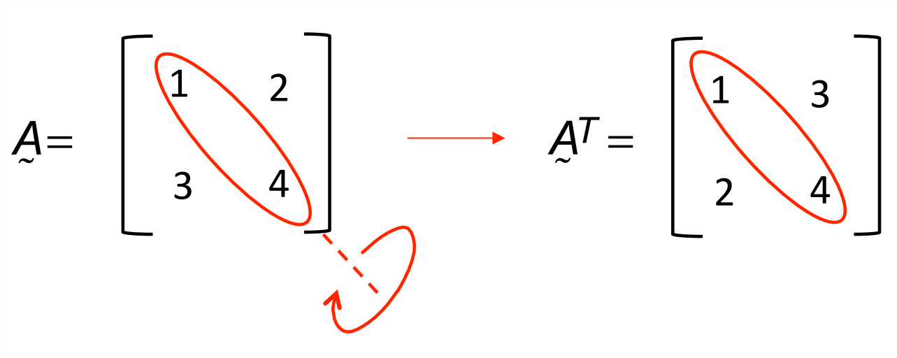
• The main diagonal of a square matrix is the collection of elements for which both indices are the same. In figure \(\PageIndex{1}\), for example, the main diagonal is outlined in red.
• The transpose of a matrix is indicated by a superscript “T”, i.e., the transpose of \(\underset{\sim}{A}\) is \(\underset{\sim}{A}^T\). To find the transpose, flip the matrix about the main diagonal: \(A_{ij}^T = A_{ji}\) as shown in figure \(\PageIndex{1}\).

Figure \(\PageIndex{1}\): Taking the transpose of a \(2\times2\) matrix.

• In a diagonal matrix, only the elements on the main diagonal are nonzero, i.e., \(A_{ij}=0\) unless \(i=j\).
• The trace is the sum of the elements on the main diagonal, i.e., \(\operatorname{Tr}(\underset{\sim}{A}) = A_{ii}\). For the example shown in figure \(\PageIndex{1}\), the trace is equal to 5. Note that \(Tr(\underset{\sim}{A}^T)=Tr(\underset{\sim}{A})\).
• For a symmetric matrix, \(\underset{\sim}{A}^T=\underset{\sim}{A}\) or \(A_{ji}=A_{ij}\). We say that a symmetric matrix is invariant under transposition. Note that a diagonal matrix is automatically symmetric.
• For an antisymmetric matrix, transposition changes the sign: \(\underset{\sim}{A}^T= −\underset{\sim}{A}\) or \(A_{ji}=−A_{ij}\).

Figure \(\PageIndex{2}\): Groups of elements to be multiplied when computing the determinant. Products of terms outlined in red are added; products in blue are subtracted. In the \(3\times3\) case, the first two columns are repeated outside the matrix.

• Identity matrix:

\[\delta_{i j}=\left\{\begin{array}{ll}
{1} & {\text { if } i=j} \\
{0} & {\text { if } i \neq j}
\end{array} \quad \text { e.g. }\left[\begin{array}{ll}
{1} & {0} \\
{0} & {1}
\end{array}\right]\right.\label{eq:5} \]

Multiplying a matrix by \(\underset{\sim}{\delta}\) leaves the matrix unchanged:\(\underset{\sim}{\delta}\underset{\sim}{A}=\underset{\sim}{A}\). The same is true of a vector: \(\underset{\sim}{\delta}\vec{v}=\vec{v}\). The identity matrix is often called \(I\).

Exercise \(\PageIndex{1}\)

Is an identity matrix diagonal?

What is the trace of a \(2\times2\) identity matrix? A \(3\times3\) identity matrix?

Is an identity matrix symmetric, antisymmetric, both, or neither?

• The determinant of \(\underset{\sim}{A}\), denoted \(\operatorname{det}(\underset{\sim}{A})\), is a scalar property that will be described in detail later (section 15.3.3). For the general \(2\times\) matrix

\[A=\left[\begin{array}{ll}
{A_{11}} & {A_{12}} \\
{A_{21}} & {A_{22}}
\end{array}\right],\label{eq:6} \]

the determinant is

\[\operatorname{det}(\underset{\sim}{A})=A_{11} A_{22}-A_{21} A_{12}. \nonumber \]

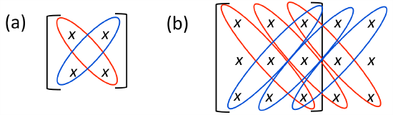
The pattern illustrated in figure \(\PageIndex{2}a\) provides a simple mnemonic. For the general \(3\times3\) matrix

\[\underset{\sim}{A}=\left[\begin{array}{lll}
{A_{11}} & {A_{12}} & {A_{13}} \\
{A_{21}} & {A_{22}} & {A_{23}} \\
{A_{31}} & {A_{32}} & {A_{33}}
\end{array}\right], \nonumber \]

the determinant is obtained by multiplying diagonals, then adding the products of diagonals oriented downward to the right (red in figure 2.3b) and subtracting the products of diagonals oriented upward to the right (blue in figure \(\PageIndex{2}b\)):

\[\operatorname{det}\left[\begin{array}{lll}
{A_{11}} & {A_{12}} & {A_{13}} \\
{A_{21}} & {A_{22}} & {A_{23}} \\
{A_{31}} & {A_{32}} & {A_{33}}
\end{array}\right]=A_{11} A_{22} A_{33}+A_{12} A_{23} A_{31}+A_{13} A_{21} A_{32}-A_{31} A_{22} A_{13}-A_{32} A_{23} A_{11}-A_{33} A_{21} A_{12} \nonumber \]

The determinant can also be evaluated via expansion of cofactors along a row or column. In this example we expand along the top row:

\[\operatorname{det}\left[\begin{array}{lll}
{A_{11}} & {A_{12}} & {A_{13}} \\
{A_{21}} & {A_{22}} & {A_{23}} \\
{A_{31}} & {A_{32}} & {A_{33}}
\end{array}\right]=A_{11} \times \operatorname{det}\left[\begin{array}{cc}
{A_{22}} & {A_{23}} \\
{A_{32}} & {A_{33}}
\end{array}\right]-A_{12} \times \operatorname{det}\left[\begin{array}{cc}
{A_{21}} & {A_{23}} \\
{A_{31}} & {A_{33}}
\end{array}\right]+A_{13} \times \operatorname{det}\left[\begin{array}{cc}
{A_{21}} & {A_{22}} \\
{A_{31}} & {A_{32}}
\end{array}\right] \nonumber \]

• Matrix inverse: If \(\underset{\sim}{A}\underset{\sim}{B}=\underset{\sim}{\delta}\) and \(\underset{\sim}{B}\underset{\sim}{A}=\underset{\sim}{\delta}\) then \(\underset{\sim}{B}=\underset{\sim}{A}^{-1}\) and \(\underset{\sim}{A}=\underset{\sim}{B}^{-1}\). For the \(2\times2\) matrix Equation \(\ref{eq:6}\), the inverse is

\[\underset{\sim}{A}^{-1}=\frac{1}{\operatorname{det}(\underset{\sim}{A})}\left[\begin{array}{cc}
{A_{22}} & {-A_{12}} \\
{-A_{21}} & {A_{11}}
\end{array}\right] \nonumber \]

Exercise \(\PageIndex{2}\)

Multiply this by \(\underset{\sim}{A}\) as given in Equation \(\ref{eq:6}\) and confirm that you get the identity matrix. Unfortunately, there is no simple formula for the \(3\times3\) case.

• Orthogonal matrix: \(\underset{\sim}{A}^{-1}=\underset{\sim}{A}^T\).

• Singular matrix: \(\operatorname{det}(\underset{\sim}{A})=0\). A singular matrix has no inverse.

Test your understanding of this section by completing exercises 2, 3, 4, 5 and 6. (Exercise 7 is outside the main discussion and can be done any time.)