
3.1: Measuring space with Cartesian coordinates
- Page ID
- 18057

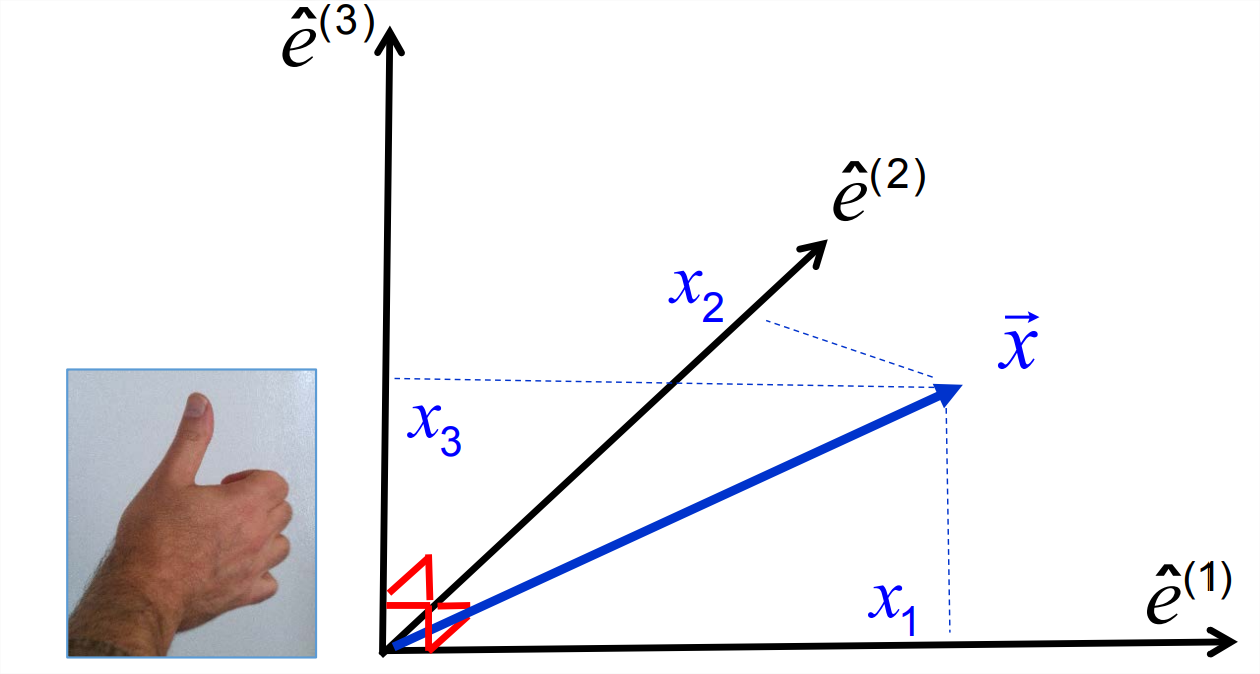
A convenient way to measure space is to assign to each point a label consisting of three numbers, one for each dimension. We begin by choosing a single point to serve as the origin. The location of any point can now be quantified by its position vector, the vector extending from the origin to the point in question. We’ll name this position vector \(\vec{x}\).
Next, choose three basis vectors, each beginning at the origin and extending away for some distance. The only real restriction on this choice is that the vectors must not all lie in the same plane. It will be easiest if we choose the basis vectors to be unit vectors, in which case we’ll name them \(\hat{e}^{(1)}\), \(\hat{e}^{(2)}\) and \(\hat{e}^{(3)}\). It’s also easiest if we choose the vectors to be mutually orthogonal:
\[\hat{e}^{(i)} \cdot \hat{e}^{(j)}=\delta_{i j}\label{eq:1} \]
Finally, it’s easiest if we choose the system to be right-handed, meaning that if you take your right hand and curve the fingers in the direction from \(\hat{e}^{(1)}\) to \(\hat{e}^{(2)}\), your thumb will point in the direction of \(\hat{e}^{(3)}\) (Figure \(\PageIndex{1}\)). Interchanging any two basis vectors renders the coordinate system left-handed. This “handedness’’ property is also referred to as parity.
Every position vector \(\vec{x}\) can be expressed as a linear combination of the basis vectors:
\[\vec{x}=x_{1} \hat{e}^{(1)}+x_{2} \hat{e}^{(2)}+x_{3} \hat{e}^{(3)}=x_{i} \hat{e}^{(i)} . \label{eq:2} \]
The component \(x_k\) can be isolated by projecting \(\vec{x}\) onto \(\hat{e}^{k}\):
\[\vec{x} \cdot \hat{e}^{(k)}=x_{i} \hat{e}^{(i)} \cdot \hat{e}^{(k)}=x_{i} \delta_{i k}=x_{k}, \nonumber \]
therefore
\[x_{k}=\vec{x} \cdot \hat{e}^{(k)}.\label{eq:3} \]
The components of the position vector are called the Cartesian coordinates of the point.
A position vector in a Cartesian coordinate system can be expressed as \(\{x_1,\,x_2,\,x_3\}\) or, equivalently, as \(\{x,\,y,\,z\}\). The numerical index notation is useful in a mathematical context, e.g., when using the summation convention. In physical applications, it is traditional to use the separate letter labels \(\{x,\,y,\,z\}\). In the geosciences, for example, we commonly denote the eastward direction as \(x\), northward as \(y\) and upward as \(z\). (Note that this coordinate system is right-handed.) Similarly, the basis vectors \(\{\hat{e}^{(1)},\,\hat{e}^{(2)},\,\hat{e}^{(3)}\}\) are written as \(\{\hat{e}^{(x)},\,\hat{e}^{(y)},\,\hat{e}^{(z)}\}\). As we transition from mathematical concepts to real-world applications, we will move freely between these two labeling conventions.
Cartesian geometry on the plane
Advanced concepts are often grasped most easily if we restrict our attention to a two-dimensional plane such that one of the three coordinates is constant, and can therefore be ignored. For example, on the plane \(x_3=0\), the position vector at any point can be written as \(\vec{x}=x_1 \hat{e}^{(1)} + x_2\hat{e}^{(2)}\), or \(\{x, y\}\). Two-dimensional geometry is also a useful first approximation for many natural flows, e.g., large-scale motions in the Earth’s atmosphere.
3.1.1 Matrices as geometrical transformations
When we multiply a matrix \(\underset{\sim}{A}\) onto a position vector \(\vec{x}\), we transform it into another position vector \(\vec{x}^\prime\) with different length and direction (except in special cases). In other words, the point the vector points to moves to a new location. Often, but not always, we can reverse the transformation and recover the original vector. The matrix needed to accomplish this reverse transformation is \(\underset{\sim}{A}^{-1}\). To fix these ideas, we’ll now consider a few very simple, two-dimensional examples.
Consider the \(2\times 2\) identity matrix \(\underset{\sim}{\delta}\). Multiplying a vector by \(\underset{\sim}{\delta}\) is a null transformation, i.e., \(\vec{x}^\prime =\vec{x}\); the vector is transformed into itself. Not very interesting.
Now consider a slightly less trivial example: the identity matrix multiplied by a scalar, say, 2:
\[\underset{\sim}{A}=\left[\begin{array}{ll}
{2} & {0} \\
{0} & {2}
\end{array}\right].\label{eq:4} \]
Solution
Multiplying \(\underset{\sim}{A}\) onto some arbitrary vector \(\vec{x}\) has the effect of doubling its length but leaving its direction unchanged: \(\vec{x}^\prime = 2\vec{x}\). Is this transformation reversible? Suppose I gave you the transformed vector \(\vec{x}^\prime\) and the transformation \(\underset{\sim}{A}\) that produced it, then asked you to deduce the original vector \(\vec{x}\). This would be very easy; you would simply divide \(\vec{x}^\prime\) by 2 to get \(\vec{x}\).
Next we’ll look at a more interesting example:
\[\underset{\sim}{A}=\left[\begin{array}{cc}
{2} & {0} \\
{0} & {1 / 2}
\end{array}\right] \label{eq:5} \]
Solution
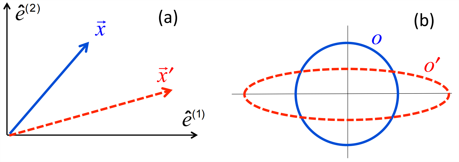
Multiplication of \(\underset{\sim}{A}\) onto any vector doubles the vector’s first component while halving its second (figure \(\PageIndex{2}a\)):
\[\text { If } \vec{x}=\left[\begin{array}{l}
{x} \\
{y}
\end{array}\right], \quad \text { then } \vec{x}^{\prime}=A \vec{x}=\left[\begin{array}{c}
{2 x} \\
{y / 2}
\end{array}\right].\label{eq:6} \]
In general, the transformation changes both the length and the direction of the vector. There are, however, exceptions that you can now confirm for yourself:
- Show that the length of a vector is not changed if its \(y\) component is \(\pm\) twice its \(x\) component.
- Identify a particular vector \(\vec{x}\) whose direction is not changed in this transformation. Now identify another one.
- Compute the eigenvectors of \(\underset{\sim}{A}\). You should find that they are simply the basis vectors \(\hat{e}^{(x)}\) and \(\hat{e}^{y}\). In general, any multiple of either of these unit vectors is an eigenvector. Note that this class of vectors is also the class of vectors whose direction is unchanged!1
Because a matrix transformation can be applied to any position vector, it can be thought of as affecting any geometrical shape, or indeed all of space. A simple way to depict the general effect of the matrix is to sketch its effect on the unit circle centered at the origin. In this case the circle is transformed into an ellipse (figure \(\PageIndex{2}b\)), showing that the general effect of the matrix is to compress things vertically and expand them horizontally.
Is this transformation reversible? Certainly: just halve the \(x\) component and double the \(y\) component. As an exercise, write down a matrix that accomplishes this reverse transformation, and show that it is the inverse of \(\underset{\sim}{A}\).
Now consider
\[\underset{\sim}{A}=\left[\begin{array}{ll}
{1} & {0} \\
{0} & {0}
\end{array}\right].\label{eq:7} \]
Solution
This transformation, applied to a vector, leaves the \(x\) component unchanged but changes the \(y\) component to zero. The vector is therefore projected onto the \(x\) axis (figure \(\PageIndex{3}a\)). Applied to a general shape, the transformation squashes it flat (figure \(\PageIndex{3}b\)). Does this transformation change the length and direction of the vector? Yes, with certain exceptions which the reader can deduce.
Is the transformation reversible? No! All information about vertical structure is lost. Verify that the determinant \(|\underset{\sim}{A}|\) is zero, i.e., that the matrix has no inverse.
Test your understanding by completing exercises (8) and (9).
As a final example, consider
\[\underset{\sim}{A}=\left[\begin{array}{cc}
{0} & {1} \\
{-1} & {0}
\end{array}\right].\label{8} \]
Solution
The matrix transforms
\[\left[\begin{array}{c}
{x} \\
{y}
\end{array}\right] \text { to }\left[\begin{array}{c}
{y} \\
{-x}
\end{array}\right]. \nonumber \]
The length of the vector is unchanged (check), and the transformed vector is orthogonal to the original vector (also check). In other words, the vector has been rotated through a \(90^\circ\) angle. In fact, it is generally true that an antisymmetric matrix rotates a vector through \(90^\circ\). To see this, apply a general antisymmetric matrix \(\underset{\sim}{A}\) to an arbitrary vector \(\vec{u}\), then dot the result with \(\vec{u}\):
\[\begin{aligned}
&(A \vec{u}) \cdot \vec{u}=A_{i j} u_{j} u_{i}=-A_{j i} u_{j} u_{i} \quad \text { (using antisymmetry) }\\
&\begin{array}{ll}
{=-A_{i j} u_{i} u_{j}} & {(\text { relabeling } i \leftrightarrow j)} \\
{=-A_{i j} u_{j} u_{i} .} & {(\text { reordering })}
\end{array}
\end{aligned} \nonumber \]
The result is equal to its own negative and must therefore be zero. We conclude that the transformed vector is orthogonal to the original vector.2
3.1.2 Coordinate rotations and the principle of relativity
It is an essential principle of science that the reality you and I experience exists independently of us. If this were not true, science would be a waste of time, because an explanation of your reality would not work on mine.
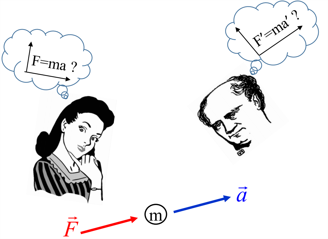
Is there any way to prove this principle? No, but we can test it by comparing our experiences of reality. For example, if you measure a force and get the vector \(\vec{F}\), and if I measure the same force, I expect to get the same result. Now, we know from the outset that this will not be quite true, because we observe from different perspectives. For example, if you see \(\vec{F}\) pointing to the right, I may see it pointing to the left, depending on where I’m standing. For a meaningful comparison, we must take account of these expected differences in perspective. Let’s call the force vector that I measure \(\vec{F}^\prime\). The components of this vector will have different values than the ones you measured (\(\vec{F}\)), but if we can somehow translate from your perspective to mine, the vectors should be the same. We expect this because the force is a physically real entity that exists independently of you and me.
Now imagine that this force acts on a mass m and we each measure the resulting acceleration: you get \(\vec{a}\) and I get \(\vec{a}^\prime\). As with the force, the components of \(\vec{a}^\prime\) will differ from those of \(\vec{a}\), but if we correct for the difference in perspective we should find that \(\vec{a}^\prime\) and \(\vec{a}\) represent the same acceleration.
Now suppose further that we are making these measurements in order to test Newton’s second law of motion. If that law is valid in your reference frame, then the force and acceleration you measure should be related by \(\vec{F}=m\vec{a}\). If the law is also valid in my reference frame then I should get \(\vec{F}^\prime=m\vec{a}^\prime\). This leads us to the relativity principle, attributed to Galileo: The laws of physics are the same for all observers. Just as with other kinds of laws, if a law of physics works for you but not for me, then it is not a very good law.
Our goal here is to deduce physical laws that describe the motion of fluids. The selection of possible hypotheses (candidate laws) that we could imagine is infinite. How do we determine which one is valid? To begin with, we can save ourselves a great deal of trouble if we consider only hypotheses that are consistent with the relativity principle. To do this, we must first have a mathematical language for translating between different reference frames. In particular, we need to be able to predict the effect of a coordinate rotation on the components of any vector, or of any other quantity we may want to work with.
3.1.3 The rotation matrix
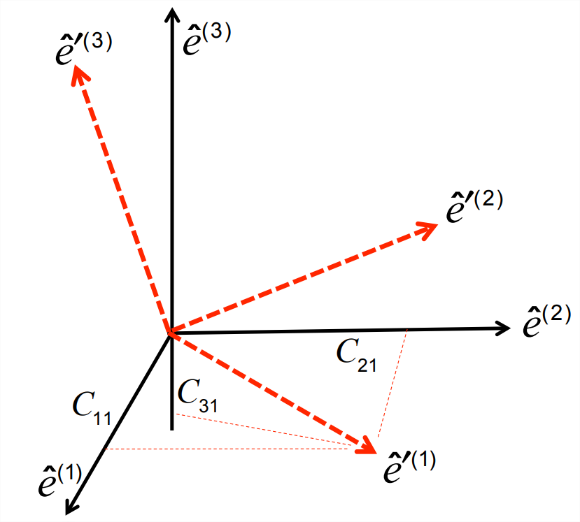
Suppose that, having defined an orthogonal, right-handed set of basis vectors \(\hat{e}^{(i)},i = 1,2,3\), we switch to a new set, \(\hat{e}^{\prime(i)}\) (figure \(\PageIndex{5}\)). Each of the new basis vectors can be written as a linear combination of the original basis vectors in accordance with Equation \(\ref{eq:2}\). For example, \(\hat{e}^{\prime(i)}\) can be written as
\[\hat{e}^{\prime (1)} =C_{i 1} \hat{e}^{(i)} \nonumber \]
This is analogous to Equation \(\ref{eq:2}\), but in this case the coefficients of the linear combination have been written as one column of a \(3\times3\) matrix \(\underset{\sim}{C}\). Doing the same with the other two basis vectors (\(\hat{e}^{\prime(2)}\) and \(\hat{e}^{\prime(3)}\) ) yields the other two columns:
\[\hat{e}^{\prime(j)}=C_{i j} \hat{e}^{(i)}, \quad j=1,2,3\label{eq:9} \]
To rephrase Equation \(\ref{eq:9}\), \(\underset{\sim}{C}\) is composed of the rotated basis vectors, written as column vectors and set side-by-side:
\[\underset{\sim}{C}=\left[\begin{array}{cc}
{\hat{e}^{\prime(1)}} & {\hat{e}^{\prime(2)}} & {\hat{e}^{\prime(3)}}
\end{array}\right]\label{eq:10} \]
Now suppose that the new basis vectors have been obtained simply by rotating the original basis vectors about some axis.3 In this case, both the lengths of the basis vectors and the angles between them should remain the same. In other words, the new basis vectors, like the old ones, are orthogonal unit vectors: \(\hat{e}^{\prime(i)}\cdot\hat{e}^{\prime(j)}=\delta_{ij}\). This requirement restricts the forms that \(\underset{\sim}{C}\) can take. Substituting Equation \(\ref{eq:9}\), we have:
\[\hat{e}^{\prime(i)}\cdot\hat{e}^{\prime(j)}=C_{ki}\hat{e}^{(k)}\cdot C_{lj}\hat{e}^{(l)}=C_{ki}C_{lj}\hat{e}^{(k)}\cdot\hat{e}^{(l)}=C_{ki}C_{lj}\delta_{kl}=C_{li}C_{lj}=C_{il}^TC_{lj}=\delta{ij}. \nonumber \]
The final equality is equivalent to
\[\underset{\sim}{C}^T=\underset{\sim}{C}^{-1}\label{eq:11} \]
i.e., \(\underset{\sim}{C}\) is an orthogonal matrix.4
Recall also that the original basis vectors form a right-handed set. Do the rotated basis vectors share this property? In section 15.3.3, it is shown that the determinant of an orthogonal matrix equals \(\pm1\). Moreover, if \(|\underset{\sim}{C}|=-1\), then \(\underset{\sim}{C}\) represents an improper rotation: the coordinate system undergoes both a rotation and a parity switch, from right-handed to left-handed. This is not usually what we want. So, if \(\underset{\sim}{C}\) is orthogonal and its determinant equals +1, we say that \(\underset{\sim}{C}\) represents a proper rotation.
To reverse a coordinate rotation, we simply use the inverse of the rotation matrix, \(\underset{\sim}{C}^{-1}\), or \(\underset{\sim}{C}^T\):
\[\hat{e}^{(j)}=C_{j i} \hat{e}^{\prime(i)}, \quad j=1,2,3 \label{eq:12} \]
Comparing Equation \(\ref{eq:12}\) with Equation \(\ref{eq:9}\), we see that, on the right-hand side, the dummy index is in the first position for the forward rotation and in the second position for the reverse rotation.
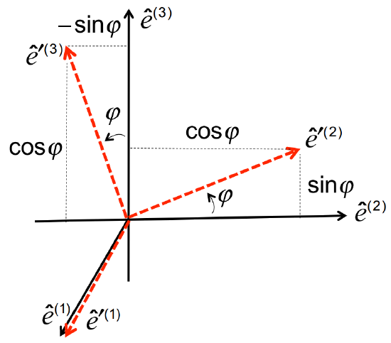
Suppose we want to rotate the coordinate frame around the \(\hat{e}^{(1)}\) axis by an angle \(\phi\). Referring to figure \(\PageIndex{6}\), we can express the rotated basis vectors using simple trigonometry:
\[\hat{e}^{\prime(1)}=\hat{e}^{(1)}=\left[\begin{array}{l}
{1} \\
{0} \\
{0}
\end{array}\right] ; \quad \hat{e}^{\prime(2)}=\left[\begin{array}{c}
{0} \\
{\cos \phi} \\
{\sin \phi}
\end{array}\right] ; \quad \hat{e}^{\prime(3)}=\left[\begin{array}{c}
{0} \\
{-\sin \phi} \\
{\cos \phi}
\end{array}\right]; \nonumber \]
Solution
Now, in accordance with Equation \(\ref{eq:10}\), we simply place these column vectors side-by-side to form the rotation matrix:
\[\underset{\sim}{C}=\left[\begin{array}{ccc}
{1} & {0} & {0} \\
{0} & {\cos \phi} & {-\sin \phi} \\
{0} & {\sin \phi} & {\cos \phi}
\end{array}\right].\label{eq:13} \]
Looking closely at Equation \(\ref{eq:13}\), convince yourself that the following are properties of \(\underset{\sim}{C}\):
- \(\underset{\sim}{C}^T\underset{\sim}{C}=\underset{\sim}{\delta}\), i.e., \(\underset{\sim}{C}\) is orthogonal.
- \(|\underset{\sim}{C}|=1\), i.e., \(\underset{\sim}{C}\) represents a proper rotation.
- Changing the sign of \(\phi\) produces the transpose (or, equivalently, the inverse) of \(\underset{\sim}{C}\), as you would expect.
Example 6: Test your understanding by completing exercise 10.
1Generalizing from this example, we could propose that an eigenvector is a vector which, when multiplied by the matrix, maintains its direction. There is a common exception to this, though, and that is when the eigenvalues or eigenvectors are complex. In that case, geometric interpretation of the eigenvectors becomes, well, complex.
2Be sure you understand this proof; there’ll be many others like it.
3The axis need not be a coordinate axis; any line will do.
4We now see why a matrix with this property is called “orthogonal”; orthogonal vectors remain orthogonal after transformation by such a matrix.