7.2: Vortex dynamics in a homogeneous, inviscid fluid

7.2.1 The vorticity equation

Assume \(\rho = \rho_0\), \(v = \rho = 0\). The mass and momentum equations Equations 6.2.5, 6.8.2 are then

\[\vec{\nabla} \cdot \vec{u}=0\label{eqn:1} \]

\[\frac{D \vec{u}}{D t}=\vec{g}-\vec{\nabla} \frac{p}{\rho_{0}}.\label{eqn:2} \]

Vorticity is defined as the curl of velocity:

\[\vec{\omega}=\vec{\nabla} \times \vec{u}.\label{eqn:3} \]

To get an equation for \(\vec{\omega}\), we take the curl of Equation \(\ref{eqn:2}\). Here are four vector identities that will be useful in that task:

1. \(\vec{\nabla} \cdot(\vec{\nabla} \times \vec{u}) \equiv 0\)
2. \(\vec{\nabla} \times(\vec{\nabla} \phi) \equiv 0\)
3. \([\vec{u} \cdot \vec{\nabla}] \vec{u} \equiv(\vec{\nabla} \times \vec{u}) \times \vec{u}+\frac{1}{2} \vec{\nabla}(\vec{u} \cdot \vec{u})\)
4. \(\vec{\nabla} \times(\vec{u} \times \vec{v}) \equiv[\vec{v} \cdot \vec{\nabla}] \vec{u}-\vec{v}(\vec{\nabla} \cdot \vec{u})-[\vec{u} \cdot \vec{\nabla}] \vec{v}+\vec{u}(\vec{\nabla} \cdot \vec{v})\)

An immediate consequence of [1] is that the vorticity field is solenoidal:

\[\vec{\nabla} \cdot \vec{\omega}=0.\label{eqn:4} \]

This is true for every flow, not just inviscid and homogeneous. Next, we apply the curl operator to Equation \(\ref{eqn:2}\), starting with the left hand side.

\[\begin{aligned}
\vec{\nabla} \times \frac{D \vec{u}}{D t} &=\vec{\nabla} \times\left(\frac{\partial \vec{u}}{\partial t}+[\vec{u} \cdot \vec{\nabla}] \vec{u}\right) \\
&=\vec{\nabla} \times\left(\frac{\partial \vec{u}}{\partial t}+\vec{\omega} \times \vec{u}+\frac{1}{2} \vec{\nabla}(\vec{u} \cdot \vec{u})\right) \\
&=\frac{\partial \vec{\omega}}{\partial t}+\vec{\nabla} \times(\vec{\omega} \times \vec{u})+0 \\
&=\frac{\partial \vec{\omega}}{\partial t}+[\vec{u} \cdot \vec{\nabla}] \vec{\omega}-0-[\vec{\omega} \cdot \vec{\nabla}] \vec{u}+0 \\
&=\frac{D \vec{\omega}}{D t}-[\vec{\omega} \cdot \vec{\nabla}] \vec{u}
\end{aligned} \nonumber \]

where the numbers indicate the vector identities employed. The right hand side is simpler:

\[\vec{\nabla} \times\left(\vec{g}-\vec{\nabla} \frac{p}{\rho_{0}}\right)=0, \nonumber \]

because the first term is a constant and the second is a gradient (see [2]). The curl of Equation \(\ref{eqn:2}\) is therefore

\[\frac{D \vec{\omega}}{D t}=[\vec{\omega} \cdot \vec{\nabla}] \vec{u}.\label{eqn:5} \]

Aside: An interesting consequence of Equation \(\ref{eqn:5}\) is that, in homogeneous, inviscid flow, if the vorticity of a fluid parcel is zero at some initial time, it remains zero for all time. Therefore if the vorticity is zero everywhere at some initial time, it remains zero everywhere, even if the flow is accelerated by gravity or pressure. This leads to the idealization of irrotational flow, in which the math is simplified by assuming that \(\vec{\omega}\) is identically zero. That idealization is useful in technological applications but less so in geophysical flows, so we will not pursue it here (for a discussion see Kundu et al. 2016).

Figure \(\PageIndex{1}\): Relative motion of two nearby fluid particles, reproduced from Figure 5.3.2).

Figure \(\PageIndex{2}\): Motion over a time increment \(\Delta t\) of points lying on a vortex filament.

7.2.2 Vortex filaments

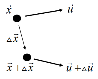
Consider, as we did previously, the relative motion of two nearby fluid particles separated by a vector \(\Delta\vec{x}\) [Figure \(\PageIndex{1}\), also see Equation 5.3.2 (5.3.1)]. The material derivative of \(\Delta\vec{x}\) is the velocity differential:

\[\frac{D}{D t} \Delta x_{i}=\Delta u_{i}=\frac{\partial u_{i}}{\partial x_{j}} \Delta x_{j}=\left[\Delta x_{j} \frac{\partial}{\partial x_{j}}\right] u_{i} \nonumber \]

or

\[\frac{D}{D t} \Delta \vec{x}=[\Delta \vec{x} \cdot \vec{\nabla}] \vec{u}.\label{eqn:6} \]

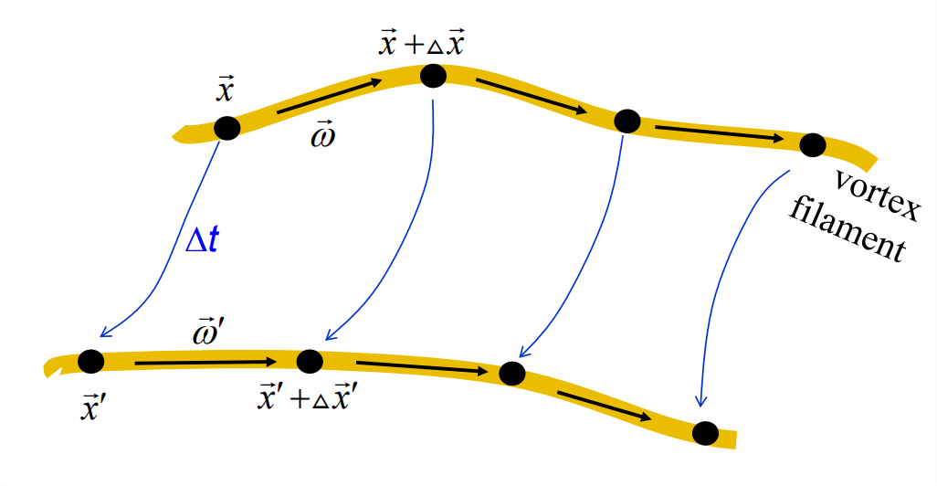
Note the correspondence in form between Equation \(\ref{eqn:5}\) and Equation \(\ref{eqn:6}\): the vorticity vector \(\vec{\omega}\) and the particle separation vector \(\Delta\vec{x}\) obey the same equation! Therefore, if \(\vec{\omega}\) and \(\Delta\vec{x}\) are parallel at some initial time, they will remain parallel for all future times. Consider the two points labelled \(\vec{x}\) and \(\vec{x}+\Delta\veC{x}\) at the upper left of Figure \(\PageIndex{2}\). These are chosen so that the separation between them, \(\Delta\vec{x}\), is parallel to the local vorticity vector \(\vec{\omega}\). After a time interval \(\Delta t\), the two points have moved to new positions \(\vec{x}^\prime\) and \(\vec{x}^\prime + \Delta\vec{x}^\prime\), and the local vorticity vector has become \(\vec{\omega}^\prime\), but the separation vector is still parallel to the vorticity.

A vortex filament is a curve within the fluid that is everywhere parallel to the local vorticity, e.g., the upper yellow curve in figure \(\PageIndex{2}\). After the time interval \(\Delta t\), each point on the vortex filament has moved to its new position, resulting in the lower yellow curve. Because the separation vector between each pair of points on the curve remains parallel to the local vorticity vector, the yellow curve remains a vortex filament. We therefore have the following theorem:

Helmholtz’s theorem #1¹

In an inviscid, homogeneous fluid, vortex filaments move with the flow.

One may say that vortex filaments are “frozen” into the flow.

Remember that the time derivative of the separation vector can also be written in terms of the the strain rate and rotation tensors (cf. 5.3.8):

\[\frac{D}{D t} \Delta \vec{x}=\Delta u_{i}=\frac{\partial u_{i}}{\partial x_{j}} \Delta x_{j}=\left(e_{i j}+\frac{1}{2} r_{i j}\right) \Delta x_{j}.\label{eqn:7} \]

It now follows from Equation \(\ref{eqn:5}\) that the same is true of the vorticity vector:

\[\frac{D}{D t} \omega_{i}=\left(e_{i j}+\frac{1}{2} r_{i j}\right) \omega_{j}.\label{eqn:8}\)

Remembering that \(r_{ij}=-\varepsilon_{ijk}\omega_j\omega_k\), we note that the second term on the right-hand side must be zero:

\[r_{i j} \omega_{j}=-\varepsilon_{i j k} \omega_{j} \omega_{k}=0, \nonumber \]

as is easily seen by interchanging \(j\) and \(k\). As a result, Equation \(\ref{eqn:8}\) becomes

\[\frac{D}{D t} \vec{\omega}=\underset{\sim}{e} \vec{\omega}.\label{eqn:9} \]

Equation \(\ref{eqn:9}\) is equivalent to Equation \(\ref{eqn:5}\)(7.2.5) , but it clearly shows the effect of strain on the vorticity.

• If the strain is extensional, it lengthens the vorticity vector just as it does the separation vector. In the ideal case where the vorticity is aligned with a principal strain, the vorticity grows exponentially, with growth rate equal to the corresponding strain rate eigenvalue. This exponential amplification of vorticity by extensional strain is called vortex stretching. Examples include tornadoes, where local rotation is amplified by stretching due to rising air, and a bathtub drain, where stretching is due to plunging water. If the local strain is compressive, the vorticity vector is compressed and its amplitude is correspondingly reduced.

The off-diagonal elements of \(\underset{\sim}{e}\) induce a tilting motion, converting one component of vorticity into another.

Figure \(\PageIndex{3}\): (a) A vorticity element (red) being tilted and stretched in a steady strain flield (blue). Numerals indicate the direction of time. (b) Counterrotating secondary vortices amplified by stretching in the extensional strain between corotating primary vortices.

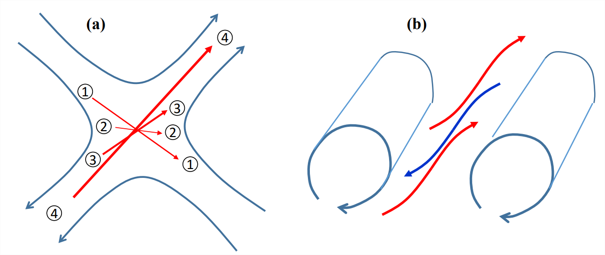
Vortex stretching is most efficient for vortices lying parallel to the principal axis of extensional strain. However, for a slowly-varying strain field, almost all vortices are rotated by the transverse strains so that they ultimately point in that optimal direction, as we now illustrate. Figure \(\PageIndex{3}\)a shows a vorticity vector (red), with material particles delineating its ends, marked “1’’. In the background is a strain field, drawn in two dimensions for simplicity. The vortex is oriented nearly parallel to the principal axes of compression. As a result, the vortex is compressed and its magnitude (speed of rotation) decreases, indicated by thinner arrow at position 2. In the next stage of evolution (position 3), the particles are drawn toward the principal axis of extension. The vorticity vector is now stretched, and its magnitude increases accordingly. Ultimately (position 4), the vortex approaches perfect alignment with the principal axis of extension. In this limit the magnitude of the vorticity grows exponentially, with growth rate equal to the largest eigenvalue of the strain rate tensor.²

While the initial prientation of the vorticity vector shown in figure \(\PageIndex{3}\)a is arbitrary, the end state is virtually always the same: the vector winds up growing exponentially in the direction of maximum extensional strain. (The only exception is if the initial vector is exactly perpendicular to the extensional strain axis, in which case it will compress to zero.)

Vortex stretching leads to a phenomenon often seen in nature - the creation of vorticity by a strain field. The flow may be almost entirely strain, but because stretched vorticity grows exponentially (in this simple geometry, at least), even a very weak vortical disturbance can rapidly become dominant. Figure \(\PageIndex{3}\)b shows a strain field between two corotating vortices. In the region between the vortices, small-amplitude vortices are stretched by the process shown in Figure \(\PageIndex{3}\)a, soon becoming aligned with the extensional strain. If you observe waves breaking on a beach, you often see that the crest of the wave just before it breaks is riven with small ripples, only an inch or so wide, aligned perpendicular to the wave crests. These are a manifestation of vortex stretching by the strain created around the wave crest as the wave grows.

7.2.3 Vorticity conservation in planar flow.

Consider a flow that lies entirely in the \(x\)−\(y\) plane, so that the vorticity is \(\omega(x,y)\hat{e}^{(z)}\). In this case the “3” component of Equation \(\ref{eqn:9}\) is

\[\frac{D}{D t} \omega=e_{3 j} \omega_{j}=\omega e_{33}. \nonumber \]

But the only nonzero components of the strain rate tensor will correspond to \(i= 1,2\) and \(j = 1,2\) (see exercise 23, for example), so that \(e_{33}=0\). As a result \(D\vec{\omega}/Dt=0.\). This result is true for all 2D flows: i.e., vorticity is conserved following the motion. There is no vortex stretching, tilting or compression in a 2D flow.

Figure \(\PageIndex{4}\): Copy and Paste Caption here

7.2.4 Vortex tubes

A vortex filament is infinitely thin, while vortices we observe have thickness. To model these, we define a vortex tube:

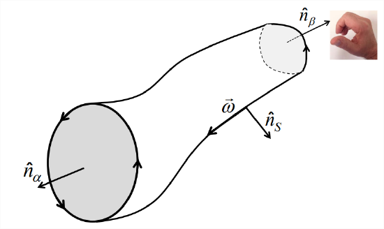
Definition: A vortex tube is a bundle of vortex filaments (Figure \(\PageIndex{4}\)).

The measure of the strength of a vortex tube is its circulation, taken around any cross section. This would not be a useful measure if it depended on the cross section chosen. Helmholtz’s theorem #2 assures us that it does not:

Helmholtz theorem #2

Circulation is the same for every cross-section through a vortex tube.

This theorem has two important corollaries:

1. Thinner parts of a vortex tube have stronger vorticity. This is because \(\Gamma = \oint \vec{\omega}\cdot \hat{n}dA\), so for \(\Gamma\) to be uniform a reduction of area must be compensated by an increase in vorticity.
2. A vortex tube cannot end within the fluid. It can either:
   • end at a boundary (e.g., tornado)
   • form a loop (e.g., smoke ring, as in Figure 7.1.1).

Proof

We will integrate the vorticity over the surface of the vortex tube segment (Figure \(\PageInde{4}\)) in two ways. First, we will perform the whole integral at once using the divergence theorem, then we will integrate over the two cross-sections and the sidewall separately. Finally we will use Stokes’ theorem to express the result in terms of circulation.

The complete integral is

\[\oint_{A} \vec{\omega} \cdot \hat{n} d A=\int_{V} \vec{\nabla} \cdot \vec{\omega} d V=0.\label{eqn:10} \]

The first equality is due to the divergence theorem; the second follows from Equation \(\ref{eqn:4}\).

Alternatively, we can perform the integral over the three surfaces seperately:

\[\oint_{A} \vec{\omega} \cdot \hat{n} d A=\underbrace{\int_{\alpha} \vec{\omega} \cdot \hat{n}_{\alpha} d A}_{=\Gamma \alpha}+\underbrace{\int_{S} \vec{\omega} \cdot \hat{n}_{S} d A}_{=0}+\underbrace{\int_{\beta} \vec{\omega} \cdot \hat{n}_{\beta} d A}_{=-\Gamma_{\beta}}=0.\label{eqn:11} \]

The first term is equal to the circulation around the cross-section \(\alpha\),

\[\Gamma_{\alpha}=\int_{\alpha} \vec{\omega} \cdot \hat{n}_{\alpha} d A, \nonumber \]

by Stokes theorem Equation 4.3.13. The integral over the sidewall (the second term) must vanish because that surface is composed of vortex filaments, and therefore its unit normal vector is everywhere perpendicular to \(\vec{\omega}\).

Stokes’ theorem requires that the unit normal be directed according to the right-hand rule, which in the third term would be into the vortex tube segment (Figure \(\PageIndex{4}\)), opposite to the outward normal \(\hat{n}\beta}\). Therefore the third term in Equation \(\ref{eqn:11}\) equals \(-\Gamma\beta\). Because the three terms must add to zero, we have \(\Gamma_\beta - \Gamma_\alpha = 0\) and the theorem is proven.

Kelvin’s circulation theorem³

If the fluid is inviscid and homogeneous, then circulation around a vortex tube does not change in time.

This explains the extraordinary longevity of vortex tubes even as they twist and turn in a turbulent flow.

Proof

As preparation, consider a scalar function of space: \(\phi = \phi(\vec{x})\). If we move through a small displacement \(d\vec{x}\), the change in \(\phi\) is

\[d \varphi=\frac{\partial \varphi}{\partial x_{i}} d x_{i}. \nonumber \]

We call this a perfect differential. Now consider the following integral

\[\int_{\vec{x}^{(1)}}^{\vec{x}^{(2)}} \frac{\partial \varphi}{\partial x_{i}} d x_{i}=\int_{\vec{x}^{(1)}}^{\vec{x}^{(2)}} d \varphi=\varphi\left(\vec{x}^{(2)}\right)-\varphi\left(\vec{x}^{(1)}\right). \nonumber \]

For a closed circuit,\(\vec{x}^{(1)}=\vec{x}^{(2)}\), and therefore

\[\oint \frac{\partial \varphi}{\partial x_{i}} d x_{i}=0. \nonumber \]

So, the integral of a perfect differential around a closed circuit is zero. Our strategy here is to get things into the form of perfect differentials.

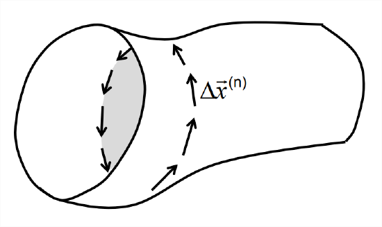
OK, here goes. Consider the circulation around an arbitrary cross-section. By the definition of the integral, we can write this as the sum over many increments, as illustrated in Figure \(\PageIndex{5}\), in the limit as the size of each increment goes to zero:

\[\Gamma=\oint \vec{u} \cdot d \vec{x}=\lim _{|\Delta \vec{x}| \rightarrow 0} \sum_{n} \vec{u}^{(n)} \cdot \Delta \vec{x}^{(n)} \nonumber \]

We now take the material derivative:

\[\begin{aligned}
\frac{D \Gamma}{D t} &=\lim _{|\Delta \vec{x}| \rightarrow 0} \frac{D}{D t} \sum_{n} \vec{u}^{(n)} \cdot \Delta \vec{x}^{(n)} \\
&=\lim _{|\Delta \vec{x}| \rightarrow 0} \sum_{n} \frac{D}{D t}\left(\vec{u}^{(n)} \cdot \Delta \vec{x}^{(n)}\right) \\
&=\lim _{|\Delta \vec{x}| \rightarrow 0} \sum_{n}\left(\frac{D \vec{u}^{(n)}}{D t} \cdot \Delta \vec{x}^{(n)}+\vec{u}^{(n)} \cdot \frac{D \Delta \vec{x}^{(n)}}{D t}\right)
\end{aligned} \nonumber \]

Now we substitute from Equation \(\ref{eqn:2}\) and return the terms to integral form

\[\begin{aligned}
\frac{D \Gamma}{D t} &=\lim _{|\Delta \vec{x}| \rightarrow 0} \sum_{n}\left[\left(\vec{g}-\frac{1}{\rho_{0}} \vec{\nabla} p^{(n)}\right) \cdot \Delta \vec{x}^{(n)}+\vec{u}^{(n)} \cdot \Delta \vec{u}^{(n)}\right] \\
&=\lim _{| \Delta \vec{x} \rightarrow 0} \sum_{n}\left[\vec{g} \cdot \Delta \vec{x}^{(n)}-\frac{1}{\rho_{0}} \vec{\nabla} p^{(n)} \cdot \Delta \vec{x}^{(n)}+\vec{u}^{(n)} \cdot \Delta \vec{u}^{(n)}\right] \\
&=\oint \vec{g} \cdot d \vec{x}-\frac{1}{\rho_{0}} \oint d p+\oint \vec{u} \cdot d \vec{u}
\end{aligned} \nonumber \]

Each of these three integrands is a perfect differential and therefore integrates to zero around a closed circuit. For clarity, we will look at the terms individually.

• The first term is the line integral of the constant vector \(\vec{g}\) around the closed curve. We could rewrite the integrand as \(g_i dx_i\), or \(d(g_ix_i)\) since \(g_i\) is a constant. So the integrand is a perfect differential.
• In the second term, \(\vec{\nabla}p^{(n)}\cdot\Delta\vec{x}^{(n)}\) has been recognized as the small change in \(p\) over the spatial increment \(\Delta \veC{x}^{(n)}\), i.e., another perfect differential.
• The third term is the perfect differential of \(\vec{u}\cdot\vec{u}/2\): \[\vec{u} \cdot d \vec{u}=u_{i} d u_{i}=u_{i} \frac{\partial u_{i}}{\partial x_{j}} d x_{j}=\frac{\partial}{\partial x_{j}}\left(\frac{u_{i}^{2}}{2}\right) d x_{j}=d\left(\frac{u_{i}^{2}}{2}\right)=d\left(\frac{\vec{u} \cdot \vec{u}}{2}\right) \nonumber \] and therefore integrates to zero.

So we have \(D\Gamma/Dt=0\), and the proof is complete.⁴

Summary: In an inviscid, homogeneous fluid we have the following:

• Helmholtz #1: Vortex tubes move with the fluid (because vortex filaments do).
• Helmholtz #2: A vortex tube cannot end within the fluid.
• Kelvin: Circulation around a vortex tube does not vary in time.

Taken together, these three theorems explain the extraordinary coherence and persistence of vortex tubes.

Figure \(\PageIndex{5}\): Line integral around a vortex tube represented as a sum of small increments.

Figure \(\PageIndex{6}\): (a) A columnar vortex tube. (b) Radial pressure variation.

7.2.5 Pressure drop within a vortex tube

Inside a vortex tube, the outward centrifugal force is balanced by a reduction of pressure. Here, we will quantify this effect.

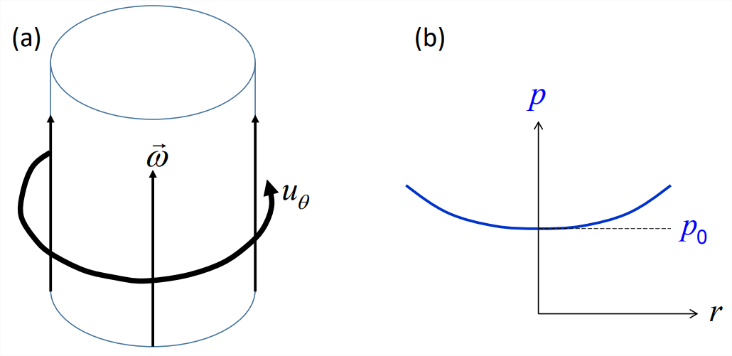
Consider a Rankine vortex with radius \(R\) in a homogeneous fluid (Figure \(\PageIndex6}\)a; also section 5.3.2). In a cylindrical coordinate system, the velocity has radial component \(u_r = 0\) and azimuthal component \(u_\theta = \dot{\theta}r\) for \(r<R\). The equation for radial velocity in this coordinate system (appendix I):

\[\frac{D u_{r}}{D t}=\frac{u_{\theta}^{2}}{r}-\frac{\partial}{\partial r} \frac{p}{\rho_{0}}.\label{eqn:12} \]

The first term on the right-hand side represents the centrifugal acceleration. To maintain \(u_r=0\), the right-hand side must vanish, i.e., the radial pressure gradient must balance the centrifugal acceleration:

\[\frac{\partial}{\partial r} \frac{p}{\rho_{0}}=\frac{u_{\theta}^{2}}{r}=\frac{(\dot{\theta} r)^{2}}{r}=\dot{\theta}^{2} r. \nonumber \]

Integrating, we have

\[\frac{p}{\rho_{0}}=\frac{1}{2} \dot{\theta}^{2} r^{2}+\frac{p_{0}}{\rho_{0}},\label{eqn:13} \]

where \(p_0\) is the pressure at \(r = 0\). The pressure profile therefore has the form of a parabola (Figure \(\PageIndex{6}\)b). The total pressure change from the center to the radius of maximum velocity (\(r = R\)) is

\[p-p_{0}=\frac{1}{2} \rho_{0} u_{\theta}^{2}, \nonumber \]

where \(p\) and \(u_\theta\) are values at \(r = R\). It is left as an exercise for the reader to determine the pressure distribution for \(r > R\). Note that \(p− p_0\) is positive definite, i.e., the pressure inside a vortex tube is always reduced.

Example: pressure drop in a tornado

A strong tornado (as defined for the purpose of nuclear reactor design) has maximum azimuthal velocity 130 m/s. Using \(ρ_0\) = 1.2 kg/m³, the mean density of air at sea level, the pressure drop is 1.4 psi, or about 1/10 of normal atmospheric pressure. This is why a tornado can cause windows to burst: on a 1 m² window, 1/10 of atmospheric pressure is about the weight of a small car.

Exercise:

Think about all the ways in which a real tornado differs from the simple model considered here.

Surface elevation in rotating flow Consider a vertical, axisymmetric vortex in homogeneous fluid with a free surface, e.g., a stirred mug of coffee. Let the height of the free surface be \(\eta(r)\). With no vertical motion, the fluid is in hydrostatic equilibrium, i.e., the pressure at each point is the weight of the fluid above it: With no vertical motion, the fluid is in hydrostatic equilibrium, i.e., the pressure at each point is the weight of the fluid above it:

\[p(r, z)=\int_{z}^{\eta(r)} \rho_{0} g d z=\rho_{0} g(\eta-z). \nonumber \]

Substitution into Equation \(\ref{eqn:13}\) gives

\[\eta=\eta_{0}+\frac{\dot{\theta}^{2}}{2 g} r^{2},\label{eqn:14} \]

where \(\eta_0\) is the surface elevation at \(r = 0\). The surface is therefore a paraboloid of revolution.⁵

Suppose we stir a cup of coffee at a rate of two revolutions per second, so that \(\dot{\theta} = 4\pi s^{-1}\). If the radius of the cup is 4 cm and \(g\) = 9.81 ms⁻², then the elevation difference should be about 1.3 cm.

You will get to play with these concepts in exercises 30 and 31.

¹Hermann von Helmholtz (1821-1894) was a German physicist and physician. He is widely known among physiologists for his work on the physics of vision. He also wrote on philosophy, particularly the relationship of perception to physical laws. A well-known partial differential equation is named for him.

²You can show this more generally by approximating \(\underset{\sim}{e}\) as a constant matrix and writing the general solution of Equation \(\ref{eqn:9}\) as a linear combination of its eigenvectors. Each coefficient grows or decays exponentially at a rate given by the corresponding strain rate eigenvalue. Eventually, the term with the largest positive eigenvalue will dominate, i.e., \(\vec{\omega}\) will approach the direction of greatest extensional strain.

³William Thompson, 1st Baron Kelvin, (1824-1907) was born in Belfast but spent most of his career at the University of Glasgow. He established the lower limit of temperature, absolute zero, and as a result the Kelvin temperature scale is named in his honor. He led the design of the first trans-Atlantic telegraph cable, for which he was knighted by Queen Victoria. He was the first British scientist elevated to the House of Lords.

⁴Note that this proof does not actually require that the path of integration enclose a vortex tube; it applies to any closed circuit in an inviscid, homogeneous fluid. The theorem also holds if \(\rho\) is not uniform provided that \(\rho\) is a function of \(p\) only, i.e., if the fluid is barotropic (see section 6.6.2).

⁵As a fluid dynamicist, always stir your coffee first and add cream second, so you can see the circulation patterns.