
4.3: Vorticity and Circulation
- Page ID
- 18062

Vorticity and circulation are two related measures of the tendency of a flow to rotate. The vorticity is the curl of the velocity field:
\[\vec{\omega}=\vec{\nabla} \times \vec{u}, \nonumber \]
or in index form
\[\omega_{k}=\varepsilon_{i j k} \frac{\partial}{\partial x_{i}} u_{j}. \nonumber \]
Using our previous formula (4.1.10) for the curl, we can write the vorticity as
\[\vec{\omega}=\hat{e}^{(x)}\left(w_{y}-v_{z}\right)+\hat{e}^{(y)}\left(u_{z}-w_{x}\right)+\hat{e}^{(z)}\left(v_{x}-u_{y}\right),\label{eqn:1} \]
where the subscripts denote partial differentiation.
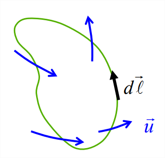
The circulation is a line integral around an arbitrarily-chosen closed curve within the space occupied by the fluid. Its value depends on the curve, velocity of the fluid on the curve, and the direction (e.g., clockwise or counterclockwise) in which the curve is traversed. The circulation is defined as
\[\Gamma=\oint \vec{u} \cdot d \vec{\ell}.\label{eqn:2} \]
4.3.1 Stokes’ theorem
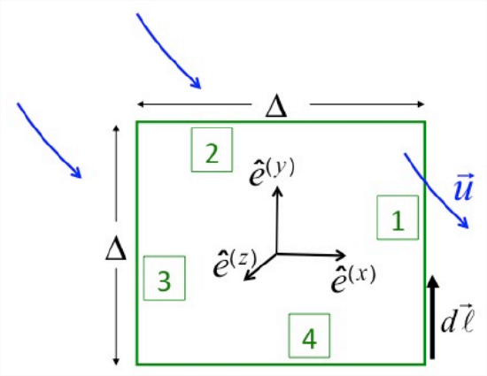
Stokes’ theorem4 makes the connection between the circulation around a curve and the vorticity within the curve. To derive Stokes’ theorem, we first evaluate the circulation around a small square (Figure \(\PageIndex{2}\)). The flow field can be three-dimensional: \(\vec{u}=\left\{u,v,w\right\}\), but the coordinates are aligned so that the square lies in the \(\hat{e}^{(x)}-\hat{e}^{(y)}\) plane. We now calculate the line integral of \(\vec{u}\cdot d\vec{\ell}\) along each of the four edges.
On edge #1, \(\vec{\ell} = \hat{e}^{(y)}\), so \(\vec{u}\cdot d\vec{\ell}=vdy\), and \(x = \Delta/2\). Expanding the spatial variation of the velocity field using a first-order Taylor series, the line integral becomes
\[\begin{align}
\Gamma^{[1]} &=\int_{-\Delta / 2}^{\Delta / 2} d y\left[v^{0}+v_{x}^{0} \frac{\Delta}{2}+v_{y}^{0} y+v_{z}^{0} 0\right] \label{eqn:3}\\
&=\left[\Delta v^{0}+\Delta v_{x}^{0} \frac{\Delta}{2}+0+0\right] \label{eqn:4}\\
&=\Delta\left(v^{0}+v_{x}^{0} \frac{\Delta}{2}\right) \label{eqn:5}
\end{align} \nonumber \]
On edge #3, \(\vec{\ell} = -\hat{e}^{(y)}\), so \(\vec{u}\cdot d\vec{\ell} = -vdy\), and \(x = −\Delta/2\). Therefore
\[\Gamma^{[3]}=-\Delta\left(v^{0}-v_{x}^{0} \frac{\Delta}{2}\right), \nonumber \]
and
\[\Gamma^{[1]}+\Gamma^{[3]}=2 \Delta v_{x}^{0} \frac{\Delta}{2}=\Delta^{2} v_{x}^{0}. \nonumber \]
Similarly,
\[\Gamma^{[2]}+\Gamma^{[4]}=-\Delta^{2} u_{y}^{0}. \nonumber \]
Adding, we get the net circulation around the square:
\[\Gamma=\Delta^{2}\left(v_{x}^{0}-u_{y}^{0}\right). \nonumber \]
Referring back to Equation \(\ref{eqn:1}\), we see that the quantity in parentheses is the z-component of the vorticity, so taking the limit \(\Delta \rightarrow 0\) we have
\[\delta \Gamma=\omega^{(z)} \delta A, \nonumber \]
where \(\delta A\) is the limit of \(\Delta^2\) and \(\omega (z) = \vec{\omega}\cdot \hat{e}^{(z)}\).
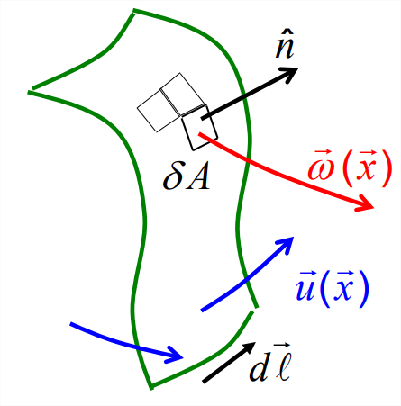
We now generalize this result to the case of an arbitrary surface. We imagine the surface as an assemblage of square tiles. The circulation around each tile is given by Equation \(\ref{eqn:1}\). As we found in the case of the volume flux (Figure 4.2.1), the line integrals along adjacent edges cancel. As a result, the net circulation is just the sum of the line integrals along the exterior edges. Summing over all of those edges in the limit as the tile size goes to zero, we have Stokes’ theorem:
Theorem: Let \(\Gamma\) be the circulation around an arbitrary closed curve \(\ell\), taken in the direction specified by the line element \(d\ell\). Moreover, let \(A\) be any surface bounded by that closed curve. The unit normal to the surface, \(\hat{n}\), is directed in accordance with the right-hand rule (with the fingers pointed along \(d\ell\)). The circulation is then given by
\[\Gamma=\oint \vec{u} \cdot d \vec{\ell}=\int_{A} \vec{\omega} \cdot \hat{n} d A.\label{eqn:6} \]