6.3: Momentum conservation

The second assumption is that momentum changes only in accordance with Newton’s second law, i.e., the rate of change of momentum of a fluid parcel equals the sum of forces applied. This assumption must be modified for relativistic flows, which occur in solar flares and supernovae, for example, but is otherwise very nearly exact.

Figure \(\PageIndex{1}\): Definition sketch for the stress vector acting across an arbitrary surface \(A\) with unit normal \(\hat{n}\).

6.3.1 Forces acting on a fluid parcel

We can write Newton’s second law for a material volume \(V_m(t)\) as an integro-differential equation analogous to Equation 6.2.1:

\[\frac{d}{d t} \int_{V_{m}} \rho \vec{u} d V=\sum_n \overrightarrow{\mathscr{F}}^{[n]}.\label{eqn:1} \]

The superscript “\(\left[ n \right]\)” is a label to enumerate the various forces that may be active. While the physical meaning of Equation \(\ref{eqn:1}\) is clear, its mathematical solution is less obvious. Our strategy is to convert it to a partial differential equation, as we did with mass conservation. First, we need to specify the individual forces \(\vec{\mathscr{F}}^{[n]}\) acting on the parcel \(V_m\). These fall into two categories: body forces and contact forces, which we now describe.

• Body forces act throughout the fluid parcel. The only body force we’ll be concerned with here is gravity.¹ We’ll assume that the gravitational field is uniform and constant, and hence can be represented by a vector \(\vec{g}\) with units of acceleration (force per unit mass). The force per unit volume is then \(\vec{F}=\rho \vec{g}\). To get the net gravitational force on a fluid parcel, we simply integrate the force per unit volume over the volume. The \(j\)-component is

\[\int_{V_{m}} \rho g_{j} d V \nonumber \]

We often work in gravity-aligned coordinates, where the direction of gravity is taken to be \(-\hat{e}^{(z)}\) (i.e., “down”), so that \(\rho\vec{g}\) becomes \(-\rho g \hat{e}^{(z)}\), \(g\) being the magnitude of \(\vec{g}\). In this case the \(j\) component of the gravitational force per unit volume is \(F_j=-\rho g \delta_{j3}\). On the Earth’s surface, a typical value for \(g\) is 9.81 ms⁻².

• Contact forces act only at the boundary of the fluid parcel. They are the macroscopic expression of intermolecular forces acting between molecules on opposite sides of the boundary. The mathematical description of these forces is one of the primary challenges of fluid dynamics, and we must overcome it before we can apply Equation \(\ref{eqn:1}\). The next subsection is devoted to the Cauchy stress tensor, through which we incorporate contact forces into Equation \(\ref{eqn:1}\).

Figure \(\PageIndex{2}\): Stress vector at a surface, with unit normal \(\vec{n}\), resolved into normal (blue) and tangential (green) components.

Figure \(\PageIndex{3}\): Stress on coordinate planes. (a) Vectors illustrate stress (force per unit area) acting on three coordinate planes. Colors indicate the force vector and the unit normal associated with each plane. (b) Array formed by the stress components, \(\tau_{ij}=f^{(I)}_j\). Normal and tangential components are colored as in Figure \(\PageIndex{2}\).

6.3.2 The Cauchy stress tensor

Imagine pushing on a solid object with your fingertip, causing it to move. You are only actually pushing on a small part of the object, namely the part in direct contact with your finger, yet the whole object moves. How? Obviously the molecules pushed directly by your finger subsequently push their neighbors, which in turn push their neighbors, and so on. If the object is a rigid solid, the force is transmitted so that all parts of the object accelerate together, greatly simplifying the application of Newton’s second law. But if the object is able to change its shape in response to your push, application of the second law presents a highly interesting challenge!

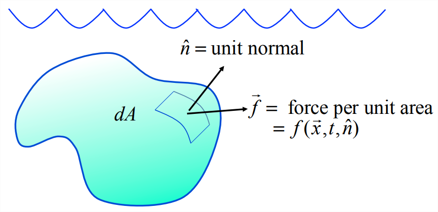
Stress is the means by which forces are transmitted through the interior of a continuous medium. A fluid is one example of a continuous medium, but the theory applies to elastic solids as well. Stress is the macroscopic expression of forces that act directly between neighboring molecules. It is the force per unit area \(\vec{f}\) acting between molecules on either side of an arbitrary surface, which may be at a physical boundary of the medium (e.g., the ocean surface) or may be an imaginary interior surface (Figure \(\PageIndex{1}\)).

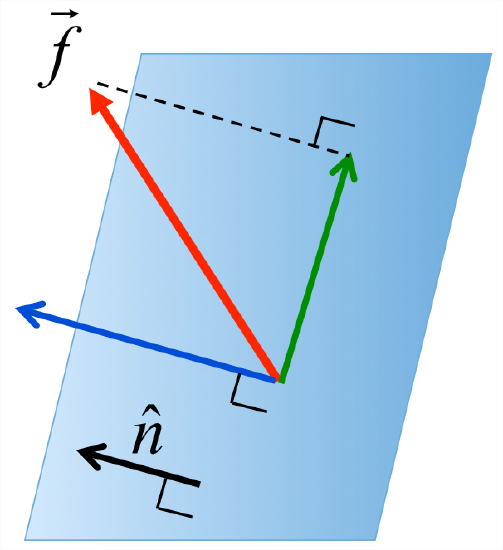
The stress vector \(\vec{f} \left( \vec{x}, t, \hat{n}\right)\) represents the force per unit area acting at a point \(\vec{x}\) on a surface where the unit normal is \(\hat{n}\) (Figure \(\PageIndex{1}\)). It is useful to think of the force as the resultant of two separate forces, one normal to the plane (Figure \(\PageIndex{2}\), shown in blue) and one tangential (green). The normal force is gotten by projecting \(\vec{f}\) onto the normal vector: \(\left( \vec{f} \cdot \hat{n}\right)\hat{n}\). The tangential is what’s left when we subtract the normal component: \(\vec{f}-\left( \vec{f} \cdot \hat{n} \right)\hat{n}\).

Some nomenclature: A normal stress may be referred to as compression (if it is directed toward the plane) or tension² (if it is directed away from the plane, as in Figure \(\PageIndex{2}\)). A tangential stress may also be called a transverse, or a shear stress. At the ocean surface, for example, the atmosphere exerts a compressive normal stress (pressure) and a tangential stress (wind).

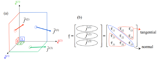
Consider the simple case of stress on a coordinate plane, a plane perpendicular to one of the basis vectors. For example, the plane labelled 1 in Figure \(\PageIndex{3}\)a (shown in blue) is perpendicular to the coordinate basis vector \(\hat{e}^{(1)}\). The stress (force per unit area) acting on this surface is defined as the vector \(\vec{f}^{(1)}\). The normal stress is \(f^{(1)}_1 \hat{e}^{(1)}\); the tangential stress is \(f_2^{(1)}\hat{e}^{(2)}+f_3^{(1)}\hat{e}^{(3)}\). Analogous vectors can be defined for the other two coordinate planes.

The three vectors \(\vec{f}^{(i)}\) have a total of 9 components which may be collected to form an array we will call the Cauchy array³:

\[\tau_{i j}=f_{j}^{(i)}.\label{eqn:2} \]

Each row of the array is one of the vectors \(\vec{f}^{(i)}\) (Figure \(\PageIndex{3}\)b). The first index of \(\tau_{ij}\)\) denotes the coordinate plane that the force acts on. The second index denotes the direction of the force component. Each element on the main diagonal represents a normal stress, while off-diagonal elements represent the tangential stresses.

Reversing Equation \(\ref{eqn:2}\), we can write the \(j\)’th component of the force on the coordinate plane whose unit normal is \(\vec{n}\) as

\[f_{j}=\tau_{i j} n_{i}.\label{eqn:3} \]

For example, if the unit normal is \(\hat{e}^{(1)}\), then \(f_j = \tau_{ij}\delta_{i1}= \tau_{1j}\).

Now suppose we could show that the Cauchy array actually transforms as a tensor. If that were true, then Equation \(\ref{eqn:3}\) could describe the force acting on any plane, because we could rotate the coordinates so that the plane in question becomes a coordinate plane and Equation \(\ref{eqn:3}\) is valid by definition. The proof that the Cauchy array is a tensor is somewhat involved. It is described in detail in appendix F. Here we give a simplified version.

Consider the net force acting on a fluid particle (a fluid parcel of infinitesimal size). In the limit as the mass becomes small, any nonzero net force results in infinite acceleration, contrary to what we observe. Therefore, the net force on a fluid particle must be zero. This is called the requirement of local equilibrium.

Figure \(\PageIndex{4}\): Two-dimensional representations of stresses acting on (a) a right triangle, (b) one corner of a rectangle. As the size of each figure goes to zero, net forces and torques must vanish.

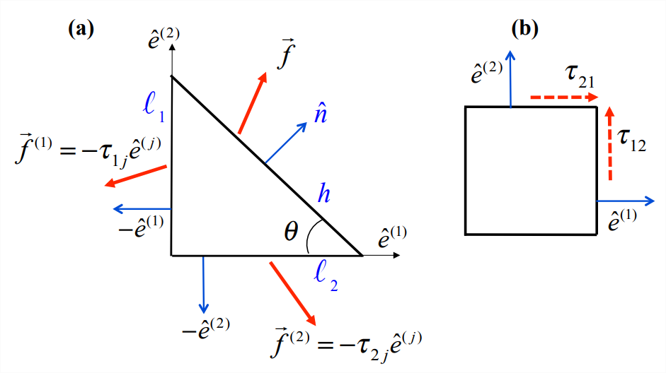
Consider a fluid parcel with the shape of a right triangle of uniform thickness, as shown on Figure \(\PageIndex{4}\)a. Look first at the left-hand face. The length of the face is \(\ell_1\), and its outward unit normal (blue arrow) is \(-\hat{e}^{(1)}\). Therefore, Equation \(\ref{eqn:3}\) tells us that the force per unit area acting on the left-hand face is \(-\tau_{1j}\hat{e}^{(j)}\). Similarly, the bottom face has length \(\ell_2\), outward normal \(-\hat{e}^{(2)}\), and force/area \(-\tau_{2j}\hat{e}^{(j)}\). Finally, let the hypotenuse have length \(h\) and force/area \(f\).

In local equilibrium, those forces balance. For the j^th component,

\[f_{j} h=\tau_{1 j} \ell_{1}+\tau_{2 j} \ell_{2}. \nonumber \]

(We have assumed that the thickness of the shape is uniform and therefore cancels out.) Now, note that \(\ell_1 = h\sin \theta\) and \(\ell_2 = h\cos \theta\); hence

\[f_{j} h=\tau_{1 j} h \sin \theta+\tau_{2 j} h \cos \theta. \nonumber \]

Dividing by \(h\) and noting that \(\hat{n}\) has components \(\{\sin \theta, \cos \theta\}\), we can write this as

\[f_{j}=\tau_{1 j} n_{1}+\tau_{2 j} n_{2}, \nonumber \]

which is equivalent to Equation \(\ref{eqn:3}\). We conclude that the stress acting at a point obeys Equation\(\ref{eqn:3}\).

Equivalently, we can say that the array \(\underset{\sim}{\tau}\) transforms as a 2nd-order tensor: \(\tau^\prime_{ij}= \tau_{kl}C_{ki}C_{lj}\). We call it the Cauchy stress tensor, or just the stress tensor. It describes a frame-independent relationship between two vectors: the force on a surface per unit area and the unit normal to that surface.

We can also show that the stress tensor must be symmetric. Consider the tangential stresses acting on two adjacent sides of a square (Figure \(\PageIndex{4}\)b). The torques exerted by these stresses act oppositely. Like the net force, the net torque must vanish as the size of the square goes to zero; otherwise there would be infinite angular acceleration. This requires that \(\tau_{12}\) and \(\tau_{21}\) be equal. By extending the argument to all three dimensions, we can show that the stress tensor at a point is symmetric (appendix F).

The symmetry of the stress tensor has three important consequences:

• The stress tensor has just six independent elements: three normal, and three tangential, to the coordinate planes.

• The formula Equation \(\ref{eqn:3}\) for the stress vector can be written in the equivalent form

\[f_{i}=\tau_{i j} n_{j},\label{eqn:4}\)

• Like the strain rate tensor (sections 5.3.3, 5.3.4), the stress tensor is a 2nd-order, real, symmetric tensor. It therefore has real eigenvalues, called the principal stresses, and real, orthogonal eigenvectors, the principal axes of stress. In the reference frame of the principal axes, the stress is entirely normal.

6.3.3 Cauchy’s equation

The net contact force on a fluid parcel is the area integral of the force per unit area (defined in 6.3.3) over the boundary:

\[\int_{A_{m}} f_{j} d A=\int_{A_{m}} \tau_{i j} n_{i} d A. \nonumber \]

The generalized divergence theorem (4.2.12) shows that the right-hand side is equal to the volume integral of the divergence of the stress tensor:

\[\int_{V_{m}} \frac{\partial \tau_{i j}}{\partial x_{i}} d V. \nonumber \]

The sum of the forces forces appearing on the right-hand side of equation Equation \(\ref{eqn:1}\) can therefore be written entirely in terms of volume integrals:

\[\frac{D}{D t} \int_{V_{m}} \rho u_{j} d V=\int_{V_{m}}\left(\rho g_{j}+\frac{\partial \tau_{i j}}{\partial x_{i}}\right) d V.\label{eqn:5} \]

Now how about the left-hand side? We can convert it to a volume integral using Equation 6.1.6 as we did in the case of mass conservation (section 6.2), but there is a very useful lemma that will make the result simpler.

Lemma

Let \(\chi\) be any quantity. Using Leibniz’s rule applied to a material volume

\[\frac{D}{D t} \int_{V_{m}} \rho \chi d V=\int_{V_{m}}\left[\frac{\partial}{\partial t} \rho \chi+\vec{\nabla} \cdot(\rho \chi \vec{u})\right] d V. \nonumber \]

Expanding via the product rule, this becomes

\[\int_{V_{m}}\left[\rho \frac{\partial \chi}{\partial t}+\chi \frac{\partial \rho}{\partial t}+\underline{\chi} \vec{\nabla} \cdot(\rho \vec{u})+\rho \vec{u} \cdot \vec{\nabla} \chi\right] d V. \nonumber \]

The second and third terms (underlined) add up to zero, as we can see by removing the common factor χ and recognizing that what’s left is the left-hand side of the mass equation 6.2.3. This leaves us with

\[\int_{V_{m}}\left[\rho \frac{\partial \chi}{\partial t}+\rho(\vec{u} \cdot \vec{\nabla}) \chi\right] d V, \nonumber \]

which you will recognize as

\[\int_{V_{m}} \rho \frac{D \chi}{D t} d V. \nonumber \]

Combining, we have

\[\frac{D}{D t} \int_{V_{m}} \rho \chi d V=\int_{V_{m}} \rho \frac{D \chi}{D t} d V.\label{eqn:6} \]

Note that this equality follows only from conservation of mass and Leibniz’s rule. Therefore, \(\chi\) can be either a scalar or a component of a vector or tensor.

Note also that Equation \(\ref{eqn:6}\) is most useful when \(\chi\) is a specific concentration, i.e., the amount of “something” per unit mass of fluid. In that case, \(\rho \chi\) is the amount per unit volume (or volumetric concentration) and the volume integral is the total amount in the fluid parcel.

Using Equation \(\ref{eqn:6}\) with \(u_j\) as \(\chi\), we can rewrite Equation \(\ref{eqn:5}\) as

\[\frac{D}{D t} \int_{V_{m}} \rho u_{j} d V=\int_{V_{m}} \rho \frac{D u_{j}}{D t} d V=\int_{V_{m}} \rho g_{j} d V+\int_{V_{m}} \frac{\partial \tau_{i j}}{\partial x_{i}} d V, \nonumber \]

or

\[\int_{V_{m}}\left\{\rho \frac{D u_{j}}{D t}-\rho g_{j}-\frac{\partial \tau_{i j}}{\partial x_{i}}\right\} d V=0 \quad \forall V_{m}. \nonumber \]

Now remember that the boundary of our fluid parcel \(V_m\) is chosen arbitrarily, so this volume integral must be zero for any fluid parcel we might choose. That can only be true if the integrand is identically zero. From this, we get the partial differential equation expressing Newton’s second law for a deformable medium, called Cauchy’s equation:

\[\rho \frac{D u_{j}}{D t}=\rho g_{j}+\frac{\partial \tau_{i j}}{\partial x_{i}}.\label{eqn:7} \]

6.3.4 Stress and strain in a Newtonian fluid

Cauchy’s equation applies not only to fluids but also to other elastic materials such as rock, metal and ice. The same theory is therefore used by seismologists, engineers, glaciologists and many others. But now we must part company with these colleagues and press on into the realm of fluids. Note that the equations we have are not closed. Cauchy’s equation represents 3 PDE’s, and we already had one from mass conservation for a total of four. But there are more unknowns than this: density, three components of velocity, plus the six independent elements of the stress tensor. To close this system, we must specify in more detail the physical nature of the material we’re talking about, and that will lead us to the idea of a “Newtonian” fluid.

We define a fluid as a material that flows in response to a shear (or transverse) stress (also see 1.2). If you apply a shear stress to a solid object it may bend or even break, but it will not flow. If it flows in response to a shear stress, it’s a fluid. This includes air, water, paint, blood, ketchup, sand, ... all of which flow in response to a shear stress, though not all in the same way. We’ll do this in two stages, talking first about a stationary (motionless) fluid, then introducing motion.

Stress in a fluid at rest

The condition for a fluid to be motionless is that there be no shear stress. In other words, the stress tensor must be diagonal, since shear stresses appear off the main diagonal. Notice, though, that the existence of shear stress depends on the choice of coordinates. Every stress tensor is diagonal in its principal coordinate frame (like the strain rate tensor as discussed in section 5.3.4). But if we rotate away from those axes, shear terms may appear off the main diagonal.

So, for a fluid to be motionless, there can be no shear stresses in any coordinate frame. This requires that the stress tensor be diagonal in every coordinate frame. This condition is satisfied only by tensors proportional to the identity tensor \(\underset{\sim}{\delta}\) (see homework problem 28), meaning that the principal stresses must all be equal. So, we’ll write the stress tensor for a motionless fluid as \(\underset{\sim}{\delta}\) times some scalar, which is the common value of the principal stresses. It will turn out to be most convenient if we build a minus sign into the definition of that scalar, so \(\underset{\sim}{\tau} = -p\underset{\sim}{\delta}\). We’ll soon recognize that the scalar \(p\) is a familiar quantity, namely the pressure. Note that the corresponding stress vector is

\[f_{j}=\tau_{i j} n_{i}=-p \delta_{i j} n_{i}=-p n_{j}, \nonumber \]

or

\[\vec{f}=-p \vec{n}. \nonumber \]

The action of pressure on any surface is normal to the surface itself.

Substituting this stress tensor into Cauchy’s equation, we have:

\[\rho \frac{D u_{j}}{D t}=\rho g_{j}-\frac{\partial p}{\partial x_{j}}, \nonumber \]

and specifying \(\vec{u} = 0\),

\[\frac{\partial p}{\partial x_{j}}=\rho g_{j}, \quad \text { or } \quad \vec{\nabla} p=\rho \vec{g}. \nonumber \]

This is the state of hydrostatic equilibrium: a balance between pressure and gravity that allows a fluid to remain motionless. In gravity-aligned coordinates, \(g_j = -g\delta_{j3}\), so:

\[\frac{\partial p}{\partial x_{j}}=-\rho g \delta_{j 3}. \nonumber \]

The pressure cannot vary in the two horizontal directions (\(j\) = 1,2, perpendicular to gravity), but varies in the vertical (\(j\) = 3) as prescribed by:

\[\frac{\partial p}{\partial z}=-\rho g.\label{eqn:8} \]

For many applications it is useful to integrate the hydrostatic equation and thereby solve for pressure:

\[p=\int_{z}^{\infty} p g d z.\label{eqn:9} \]

This tells us that the pressure at height \(z\) equals the weight of all fluid above \(z\). In the atmosphere, \(\rho \sim\) 1.2 kg/m³ at sea level and decreases to unmeasureably small values a few tens of kilometers up. The SI unit for pressure is Newtons per square meter, i.e., force per unit area (which makes sense because it is a stress.) An abbreviation for this unit is the pascal (Pa). At sea level, the mean atmospheric pressure is about 105 Pa, which is sometimes referred to as one bar. Meteorologists express pressure in millibars, so mean surface pressure is 1000 mbar. The old unit for pressure, which is still in common use, is pounds per square inch, or psi. Mean atmospheric pressure at the surface is 14 psi.

A well-inflated car tire holds about 28-30 psi in excess of the external (atmospheric) pressure, while pressures in bike tires can be as much as 130 psi. Pressurized tires maintain their shape thanks to Pascal’s Law: pressure acts equally in all directions. This is just another way to say that, in hydrostatic equilibrium, the stress tensor is isotropic. The force (per unit area) is \(f_j = n_i\tau_{ij} = n_i(-p\delta_{ij}) = -pn_j\), so it acts opposite to the outward normal from any surface (real or fictitious) regardless of its orientation.

In oceanography, we usually define a Cartesian coordinate system such that \(z\) = 0 is at the ocean surface, and \(z\)-values in the ocean are therefore negative. The pressure is given by Equation 8.2.3, but we can now break the range of integration into two parts; the integral from \(z\) to 0 (the ocean surface) and the integral from 0 to infinity, which is just atmospheric pressure at the surface. So pressure beneath the ocean surface is the sum of atmospheric pressure and the weight of the water above a given depth:

\[p=\int_{z}^{0} \rho_{w a t e r} g d z+\int_{0}^{\infty} \rho_{a i r} g d z.\label{eqn:10} \]

Stress in a moving fluid

“Air, I should explain, becomes wind when it is agitated.” - Titus Lucretius Carus, On the Nature of Things

We now allow our fluid to flow. To begin, we’ll define a new quantity, a tensor expressing the added stress due to the fact that the fluid is in motion, i.e.

\[\tau_{i j}=-p \delta_{i j}+\sigma_{i j}.\label{eqn:11} \]

This new tensor \(\sigma\) is called the “deviatoric” stress tensor. Despite the complicated name, this stress is familiar; it’s basically just friction.⁴

And how do we write the deviatoric stress tensor? To do that, we need to specify the kind of fluid we’re talking about, because deviatoric stress is different in different fluids. Remembering that deviatoric stress is just friction, you can imagine that it would be different in gooey maple syrup than in thin air, and the differences actually get more complicated than that.

We will now make a sequence of three assumptions that define a hypothetical substance called Newtonian fluid. These will be labelled N1, N2 and N3.

Assumption N1: The deviatoric stress depends only on the velocity gradient tensor. Is this assumption plausible? Yes, it makes intuitive sense that friction should depend on differences of velocity between different fluid parcels.

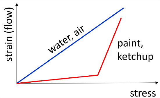
Assumption N2: Deviatoric stress is a linear function of the velocity gradients. This is best understood in terms of a counterexample: paint (Figure \(\PageIndex{5}\)). Paint is manufactured so that, when you apply stress to it using your paintbrush, it flows easily. But after it’s on the wall, the stress applied by gravity tends to make it run (i.e., strain), and you want to minimize that. So good quality paint has a nonlinear relationship between stress and strain, maximizing strain under the strong stress of the brush, but minimizing it under the weak stress of gravity. The same is true of ketchup. In an old-fashioned glass bottle, mild shaking causes the ketchup to stay right where it is. But if you shake harder, you reach a threshold where suddenly the ketchup flows, typically onto your shirt. So the assumption we’re making here is that we’re NOT talking about paint or ketchup, we’re talking about a fluid in which strain increases with stress at a uniform rate. In this case we can write the stress-strain relationship using a 4-dimensional tensor:

\[\sigma_{i j}=K_{i j k l} \frac{\partial u_{k}}{\partial x_{l}}.\label{eqn:12} \]

You can also think of this as the first term in a Taylor series approximation of a more general function consistent with N1. In that case, we expect Equation \(\ref{eqn:12}\) to be valid for velocity gradients that are not too intense.

But how do we write \(K\)? Note that we seem to be going in the wrong direction: we started with 10 unknowns, and we have just added another 81! Bear with me.

Assumption N3: The fluid is “frictionally isotropic”, i.e., friction acts the same in every direction. A counterexample to this would be blood, which has platelets in it that cause the fluid to flow more easily in some directions than in others. So, if we are not dealing with paint, ketchup, blood or the like, we can assume that the deviatoric stress and the strain are connected by a 4-dimensional tensor \(K\) that is isotropic. In that case, the most general form for \(K\) is

\[K_{i j k l}=\lambda \delta_{i j} \delta_{k l}+\mu \delta_{i k} \delta_{j l}+\gamma \delta_{i l} \delta_{j k},\label{eqn:13} \]

where \(\lambda\), \(\mu\) and γ are scalars (appendix C).

So a Newtonian fluid is defined by the assumption that deviatoric stress tensor is proportional to strain tensor, and the 4-dimensional tensor of proportionality constants is isotropic. How does this make life better? Well, we’ve just reduced 81 unknowns to 3: \(\lambda\), \(\mu\) and \(\gamma\). But we can do even better.

We already know is that the stress tensor is symmetric, and therefore so is the deviatoric stress tensor. From Equation \(\ref{eqn:12}\), it is obvious that \(\underset{\sim}{K}\) is symmetric in its first and second indices. Knowing this, we can now show that \(\gamma\) and \(\mu\) are the same. Working from Equation \(\ref{eqn:13}\), we write

\[\begin{aligned}
K_{i j k l}-K_{j i k l} &=0 \\
&=\lambda\left(\delta_{i j}-\delta_{j i}\right) \delta_{k l}+\mu\left(\delta_{i k} \delta_{j l}-\delta_{j k} \delta_{i l}\right)+\gamma\left(\delta_{i l} \delta_{j k}-\delta_{j l} \delta_{i k}\right).
\end{aligned} \nonumber \]

The first term on the right-hand side is zero because \(\delta\) is symmetric. The products of \(\delta\)’s in the second term are the same as those in the third, just reversed; hence:

\[K_{i j k l}-K_{j i k l}=(\mu-\gamma)\left(\delta_{i k} \delta_{j l}-\delta_{j k} \delta_{i l}\right)=0.\label{eqn:14} \]

Note that this equation holds for every combination \(ijkl\). The expression \(\delta_{ik}\delta_{jl}-\delta_{jk}\delta_{il}\) on the right hand side will be zero for some such combinations, but not for all. The only way that Equation \(\ref{eqn:14}\) can hold for all \(ijkl\) is if \(\mu - \gamma = 0\).

As a result, Equation \(\ref{eqn:13}\) becomes

\[K_{i j k l}=\lambda \delta_{i j} \delta_{k l}+\mu\left(\delta_{i k} \delta_{j l} \mp \delta_{i l} \delta_{j k}\right),\label{eqn:15} \]

eliminating one more unknown.

We can now substitute Equation \(\ref{eqn:15}\) in Equation \(\ref{eqn:12}\):

\[\begin{aligned}
\sigma_{i j} &=K_{i j k l} \frac{\partial u_{k}}{\partial x_{l}} \\
&=\lambda \delta_{i j} \delta_{k l} \frac{\partial u_{k}}{\partial x_{l}}+\mu\left(\delta_{i k} \delta_{j l}+\delta_{i l} \delta_{j k}\right) \frac{\partial u_{k}}{\partial x_{l}} \\
&=\lambda \delta_{i j} \frac{\partial u_{k}}{\partial x_{k}}+\mu\left(\frac{\partial u_{i}}{\partial x_{j}}+\frac{\partial u_{j}}{\partial x_{i}}\right) \\
&=\lambda \delta_{i j} e_{k k}+2 \mu e_{i j}.
\end{aligned} \nonumber \]

We now substitute this result into Equation \(\ref{eqn:11}\), arriving at

\[\tau_{i j}=-p \delta_{ij}+\lambda \delta_{ij} e_{k k}+2 \mu e_{i j} \label{eqn:16} \]

This is an example of a constitutive relation. A fluid that obeys this particular constitutive relation is called a Newtonian fluid. Air and water are Newtonian to a very close approximation; ketchup is not. Before we substitute our stress tensor back into the Cauchy equation, let us look at the two new parameters that have appeared: \(\mu\) and \(\lambda\). Each represents a different kind of friction. The term involving \(\mu\) contains \(e_{ij}\), which you will recall is the symmetric part of the velocity gradient tensor. The quantity \(\mu\) is called the dynamic viscosity. Dynamic viscosity depends on temperature, but in many real-life situations it is nearly constant. Typical values are

\[\mu=\left\{\begin{array}{ll}
10^{-3} k g m^{-1} s^{-1}, & \text {in water } \\
1.7 \times 10^{-5} k g m^{-1} s^{-1}, & \text {in air.}
\end{array}\right.\label{eqn:17} \]

The quantity \(\lambda\) is called the “second viscosity’’. As with pressure, the stress involving \(\lambda\) is proportional to the identity tensor, and therefore involves purely normal stresses. Moreover, it is proportional to \(e_{kk} = \vec{\nabla}\cdot\vec{u}\). This friction responds to either expansion or contraction of the fluid, and is zero in an incompressible fluid. The second viscosity term is negligible in most applications to the atmosphere and oceans. Before long we are going to assume that it is zero and forget about it, but we can easily go back and retrieve it should we ever want to.

Figure \(\PageIndex{5}\): Schematic examples of constitutive relationships between stress and strain.

6.3.5 The Navier-Stokes equation

Now we can substitute the Newtonian stress tensor Equation \(\ref{eqn:16}\) into Cauchy’s equation Equation \(\ref{eqn:7}\). For the special case of uniform \(\lambda\) and \(\mu\), the result is

\[\begin{align}
\rho \frac{D u_{j}}{D t} &=\rho g_{j}+\frac{\partial}{\partial x_{i}} \tau_{i j} \\
&=\rho g_{j}+\frac{\partial}{\partial x_{i}}\left[-p \delta_{i j}+\lambda \delta_{i j} e_{k k}+\mu\left(\frac{\partial u_{i}}{\partial x_{j}}+\frac{\partial u_{j}}{\partial x_{i}}\right)\right] \\
&=\rho g_{j}-\frac{\partial p}{\partial x_{j}}+\lambda \frac{\partial}{\partial x_{j}} e_{k k}+\mu \frac{\partial^{2} u_{j}}{\partial x_{i}^{2}}+\mu \frac{\partial^{2} u_{i}}{\partial x_{j} \partial x_{i}}\label{eqn:18}
\end{align} \nonumber \]

This is called the Navier-Stokes equation, and it’s the central equation of fluid dynamics. In vector form it looks like this:

\[\rho \frac{D \vec{u}}{D t}=\rho \vec{g}-\vec{\nabla} p+\mu \nabla^{2} \vec{u}+(\lambda+\mu) \vec{\nabla}(\vec{\nabla} \cdot \vec{u})\label{eqn:19} \]

The final two terms on the right-hand side have been interchanged for clarity. For incompressible flow, the final term vanishes.

To summarize, the Navier-Stokes equation Equation \(\ref{eqn:19}\) describes how the velocity at a point evolves in response to four forces, corresponding to the four terms on its right-hand side:

• Gravity acts just as it does on solids.

• The pressure gradient force acts oppositely to the gradient of the pressure, pushing fluid from high- to low-pressure regions.

• The viscosity term represents the effect of friction as neighboring molecules collide. This tends to smooth out gradients in the velocity.

• The fourth term, nonzero only in compressible flow, describes viscous resistance to either expansion or contraction.

Test your understanding: It is important that you understand the assumptions that had to be made to arrive at Equation \(\ref{eqn:19}\). Go back through section 6.3 and identify the parts that were essential for this argument. Then list as many circumstances as you can think of in which Equation \(\ref{eqn:19}\) would not be valid.

6.3.6 Eddy viscosity

We think of viscosity as being due to molecular forces but it is also useful to think of it as being due to turbulence. Turbulence can be considered a phenomenon separate from the “main” flow. For example, flow over an airplane wing is smooth up to a certain speed, after which it develops little swirls and eddies. The “main” flow still goes over the wing, but it has this added, small-scale component. Turbulent eddies exert a drag on the plane, very similar to friction. To the pilot, it feels like the air has become more viscous. Models of this effect are essential in the design of airplane wings. Turbulence modeling is also necessary in every atmospheric and ocean model.

To use such a model, we define an “effective” viscosity (or eddy viscosity) due to turbulence. This “viscosity” is usually much greater than the molecular viscosity. In the simplest models, eddy viscosity is assumed to be a constant. But it is much more accurate to let eddy viscosity vary in space and time in response to changes in the large-scale flow. This requires re-deriving Equation \(\ref{eqn:18}\) and Equation \(\ref{eqn:19}\) with derivatives of \(\mu\) and \(\lambda\) retained. A further generalization recognizes that turbulence may not be isotropic. In that case, assumption N3 must be revisited. We will normally assume that eddy viscosity is a scalar constant, like molecular viscosity.

¹Electromagnetic forces are another example of a body force. Their inclusion leads one into the fascinating realm of magnetohydrodynamics, which is unfortunately beyond our scope here (but see Choudhuri 1996).

²This is the origin of the word “tensor”.

³Augustin-Louis Cauchy (1789-1857) was a French mathematician who pioneered group theory and complex analysis, as well as many areas of mathematical physics including the one we are interested in here: the mechanics of deformable materials. He is reputed to have more concepts and theorems named after him than any other mathematician, and you will see evidence of this.

⁴Note also that, in this definition, the pressure \(p\) need not be in hydrostatic balance.