
2.5: Noise Modeling - White, Pink, and Brown Noise, Pops and Crackles
- Page ID
- 22368

Introduction
Noise is all around us in all sorts of forms. In the common use of the word, noise refers to sound. However, noise can more accurately be thought of as random variations that are always present in one or more parts of any entity such as voltage, current, or even data. Rather than thinking of noise only as an acoustic term, it should be thought of more as a random signal. Noise can be the inherent fluctuations in some part in a system (ie. temperature at a given point) or it can be the unavoidable interference on a measurement from outside sources (ie. vibrations from a nearby generator blur measurements from a pressure transducer). The static interference on your radio, the ‘snow’ on your television, and the unresolved peaks on an infrared spectroscopy report are all examples of noise.
Chemical engineers can use statistical properties to characterize noise so they can understand a current process or develop an optimal process. By characterizing the noise and determining its source, the engineer can devise methods to account for the noise, control a process, or predict the path of a system. For example, when chemical engineers design plants, they use characterizations of noise to determine the best control scheme for each process. Mathematical modeling can be used to characterize and predict the noise of a given system. In modeling, to simplify the representation of general trends that reoccur, noise is classified in two major categories: frequency based and non-frequency based. Frequency based noise consists of the colors of noise, and non-frequency based noise includes pops, snaps and crackle.
The purpose of the following sections is to give you a qualitative understanding of the sources of noise and how it can be characterized and handled. Examples will be given to help you gain a quantitative understanding of how noise relates to controlling and modeling chemical engineering processes.
General Types of Noise
Three general types of noise can be categorized in describing a process, and are as follows:
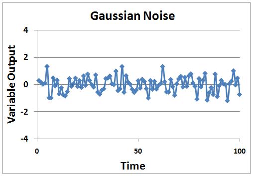
1) Gaussian noise is usually not dependent on time, meaning that it is random and not systematically planned. The amplitude of the frequency can vary, making a crackling notation or sound (see #Crackles below). Some examples of Gaussian noise can include splashing in a tank or unplanned interruption in a sensing device.
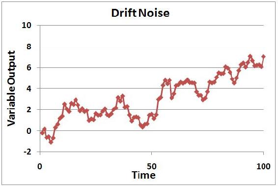
2) Drift noise is correlated to time, and has random movement. Examples of drift noise can include fouling or catalyst decay, in which the potency of the substance may decline over time as decaying occurs. Stock price fluctuations also model somewhat like drift noise.
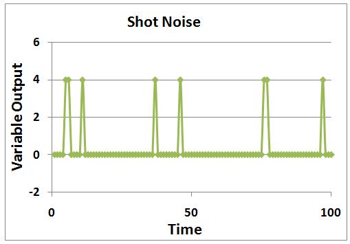
3) Shot noise may be defined as sporadic and short bursts of noise, in which the amplitude is similar among the bursts of noise. Shot noise can be correlated to pops (see #Pops below), in which at random times, the same shot noise is witnessed with the same amplitude. Examples of shot noise include partial clogging or jamming in the process in which the same amplitude will be seen by the noise whenever the clogging or jamming in the process occurs. Another example is customer demand of the product. If the control system (when trying to optimize it) depends on the customer order, and customer demand is not consistent at all times (meaning downtimes for orders) but the order amount is the same when orders are placed, then it will be effected by the shot noise described by the customer order (customer demand).
Microsoft Excel Formulas for 3 Types of Noise
| Noise Type | Excel Formula |
|---|---|
| Gaussian Noise | = [Original value] + RAND() - RAND() + RAND() - RAND()1 |
| Drift Noise | = [Previous value] + RAND() - RAND() + RAND() - RAND()1 |
| Shot Noise | = if(RAND()>0.9, [Original value]+[single error], [Original value]) |
1The more add/subtract cycles of RAND() you use, the closer approximation you'll get for a Gaussian distribution
of random errors.
As you would see these in an Excel file:
| \ | A | B | C | D |
|---|---|---|---|---|
| 1 | Time | Gaussian Noise | Drift Noise | Shot Noise |
| 2 | 1 | original value | original value | original value |
| 3 | 2 | = $B$2 + RAND() - RAND() + RAND() - RAND() | = C2 + RAND() - RAND() + RAND() - RAND() | = if(RAND()>0.9, $D$2+[single error value], $D$2) |
| 4 | 3 | = $B$2 + RAND() - RAND() + RAND() - RAND() | = C3 + RAND() - RAND() + RAND() - RAND() | = if(RAND()>0.9, $D$2+[single error value], $D$2) |
Note: These formulas can be extended for any length of time. Longer periods of time are useful for visualizing drift noise.
Combined Types of Noise
Sensors, processes, demands, etc. often do not behave with simple noise models. However, most noise can be derived from the three general types of noise. An example of a process with random and shot noise is shown in the thumbnail.
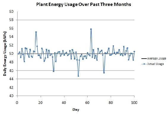
This is a graph of the total daily electricity usage for a plant during a normal operation period. As we can see, there are minor fluctuations occurring every day, but some days there are large changes of electricity usage. These large changes can be seen as shot noise when the consumption is viewed on this daily scale.
Possible reasons for the minor fluctuations could be due to electric heaters kicking on and off. Changes in the operation of smaller pumps can cause these changes in electricity demand.
The large shots could be due to an energy-intensive part of the process that only operates when needed. The positive shots could be due to this process kicking on and the negative shots could be due to a large process kicking off when not needed.
With this graph, we can say that there is shot noise present with the large changes in consumption, but there is also random noise present with the minor daily fluctuations. We would not say there is drift noise present because the consumption remains around a constant mean value and does not drift away from there.
However, the total consumption when viewed from a different scale may show other forms of noise. If we viewed the hourly usage of electricity on one of the days with shot noise, it may resemble drift noise on the hourly scale.
Colors of Noise
The first category of noise is frequency-based noise, classified by the colors of noise. In understanding the colors of noise, we need to understand the process of converting a given set of data to a point where it can be classified as some color of noise. The section below, “Modeling Noise,” goes into more detail as to how this is done. At this point, it is important to understand the main colors of noise which are possible in a system. Noise is classified by the spectral density, which is proportional to the reciprocal of frequency (\(f\)) raised to the power of beta. The power spectral density (watts per hertz) illustrates how the power (watts) or intensity (watts per square meter) of a signal varies with frequency (hertz).
\[P S D \propto \frac{1}{f^{\beta}} \nonumber \]
where \(β \ge 0\).
Just like colors of light are discriminated by their frequencies, there are different colors of noise. Each beta value corresponds to a different color of noise. For example, when beta equals zero, noise is described as white and when beta equals two, noise is described as brown.
White Noise
One major type of noise is white noise. A defining characteristic of this type of noise is it has a flat power spectral density, meaning it has equal power at any frequency. \(β\) equals zero for white noise.
White noise and white light have similar properties. White light consists of all visible colors in the spectrum while white noise is created by combining sounds at all different frequencies. Pure white noise across all frequencies cannot physically exist. It requires an infinite amount of energy and all known energy is finite. White noise can only be created within a specific and defined range of frequencies. Again making an analogy to white light, for a small band of frequencies, visible white light has a flat frequency spectrum. Another property of white noise is that it is independent of time. This factor also contributes to the idea that white noise cannot physically exist since it is impossible to have noise be completely independent of time.
A sample power spectral density chart of white noise is shown below. As can be seen from the chart, the power over all displayed frequencies is essentially the same, suggesting the PSD is equal to 1.
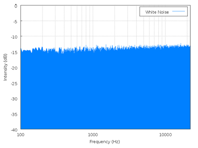
image from en.Wikipedia.org/wiki/White_noise on 9/18/2006
It is important to note that white noise is not always Gaussian noise. Gaussian noise means the probability density function of the noise has a Gaussian distribution, which basically defines the probability of the signal having a certain value. Whereas white noise simply means that the signal power is distributed equally over time. For Gaussian white noise one finds the number of measurements greater than the power spectral line as measurements that are less than the power spectral line with majority falling at the spectral line. Gaussian white noise is often used as a model for background noise in satellite communication. White noise can also come from other distributions, such at the Poisson distribution. Poissonian white noise will look like a normal distribution that has been shifted to the left for small number of measurements. For larger number of measurements Poissonian white noise will look like the normal distribution (also known as gaussian white noise). A Poissonian white noise model is useful for systems where things happen in discrete amounts such as photons being transmitted or the number of cars that go through an intersection.
Pink Noise
Pink noise is a signal whose power spectral density decreases proportionally to the inverse of the frequency, where the β value is equal to one. Because of its decrease in power at lower frequencies when compared to white noise, pink noise often sounds softer and damper than white noise.
Pink noise is actually what is commonly considered audible white noise and is evident in electrical circuits. Pink noise becomes important to measure in things such as carbon composition resistors, where it is found as the excess noise above the produced thermal noise. Below is a power spectral density chart for Pink noise.
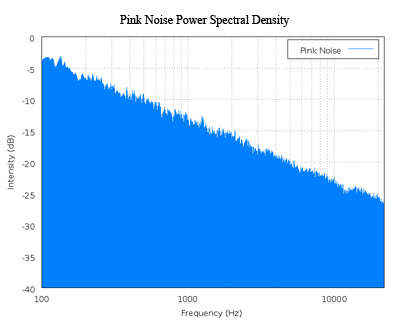
image from en.Wikipedia.org/wiki/Pink_noise on 9/18/2006
Brown Noise
When \(β\) equals 2, the noise is Brownian. Brown noise is signal noise created by Brownian, or random, motion. It is a form of unavoidable interference in the transmission of information and can be compared to a random walk that does not have a clearly patterned path. Brown noise has more energy at lower frequencies. Compared to white or pink noise, brown noise is even more soft and damped. It can be generated by integrating white noise. Interference from outside sources, such as vibrations from nearby machinery or background light, in instrument readings usually have a brown noise pattern.
Below is a power spectral density chart for brown noise. From the charts of brown noise and pink noise, it can be observed that brown noise loses power as frequency increases at a much faster rate than that of pink noise.
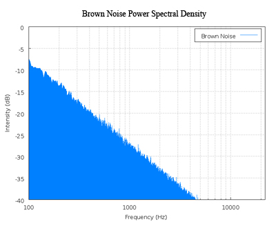
image from en.Wikipedia.org/wiki/Brown_noise on 9/18/2006
Blue Noise
Blue noise is a signal whose power spectral density increases proportionally to the frequency, where the β value is equal to negative one. An example of would be a reversible, exothermic, batch reaction where the products are being accumulated at an overall constant rate, but the reverse reaction occurs when the temperature gets too high. Thus it is overall increasing in product, but has small fluctuations as it increases. Below is a power spectral density chart for blue noise.
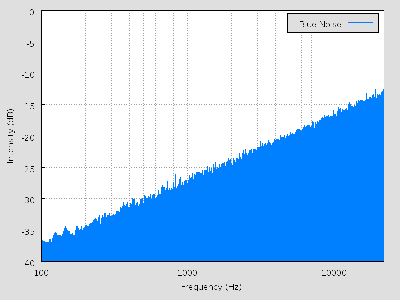
image from en.Wikipedia.org/wiki/Blue_noise#Blue_noise on 12/11/2008
Purple Noise
When β equals -2, the noise is violet. Purple noise has more energy at higher frequencies. It can be generated by differentiating white noise. Below is a power spectral density chart for purple noise. From the charts of purple noise and blue noise, it can be observed that purple noise gains power as frequency increases at a much faster rate than that of blue noise.
Modeling Colors of Noise
Characterizing noisy signals is important to a chemical engineer so that he or she can determine the sources of noise and how to account for it. Sometimes, the noise will be a characteristic of the system. In these cases, the system can not have a very sensitive control because if the sensor for the controlling device is too sensitive, it will respond to the noise of your system and end up controlling your system in a noisy way. Other times, the noise will be from unavoidable disturbances to the system. In these cases, the noise can be damped or accounted for in an appropriate manner.
In order to apply the knowledge of the colors of noise we need to understand the process of converting a given set of data to a point where it can be classified as some color of noise. The general process of classifying noise follows.
Data  Curve to Fit Data Fourier Transform Power Spectral Density Classification of Noise Color
The classification of noise color becomes important when we need to have an estimate of future data. In other words, given the trends in our current data we can use it to estimate future data. This is done as follows,
Noise Color Power Spectral Density Fourier Transform Curve Generate Data From Curve
The power of a noise signal is detected at a certain frequency. Then a plot of the log(power) vs. the log(frequency) can be constructed, and the slope of the line gives the beta value. Following a backward thought process, one can produce a certain color of noise by creating frequency components which have a value generated by a Gaussian distribution and then scaling by the appropriate beta power of frequency.
A general method to characterize and model noise is explained below.
1. DATA
Data is what the signal transmits. The signal is dependent on what you are measuring or modeling. The data can be collected, for example, if you're measuring temperature in a reactor, then your data is the temperature readings from a thermocouple at a certain position in the reactor over a period of time.
2. CURVES
After you collect the data, you plot the data and find a best fit equation,  , for that set of data. A math program can be used to find a best fit equation. Microsoft Excel can be used for a simple model and programs such as Polymath or Mathematica can be used for more complex models. A simple equation could be in the form of
  . The coefficients A and B can be varied to fit the data. Additional terms can be added for more accurate modeling of complex data. The equation you find can then be used to predict and model future signal noise.
3. FOURIER TRANSFORMS
A Fourier transform is a tool used to convert your data to a function of  . In this form, the noise can be more easily characterized. Apply a Fourier transform to the curve,, you fit to your data to generate a relation for the power spectral density. The Fourier transform can be performed by a computer depending on the complexity of (or see "Simplifying the Fourier Transform" below). The transform is the integral shown below.
\[X(w)=\int_{-\infty}^{\infty} x(t) e^{-j w t} d t \nonumber \]
where;
- is the equation of the curve to fit the data.
 is the exponential form of writing the relation
  . The j in the second term here indicates that that term is imaginary.
  is the frequency
4. POWER SPECTRAL DENSITY
This value is attained by simplifying and squaring the Fourier Transform. Since the series of simplifications needed are fairly complex, the resulting power spectral density equation is displayed below.
\[P S D=\sqrt{\left(\sum x(t) \cos (w t)\right)^{2}+\left(\sum x(t) \sin (w t)\right)^{2}} \nonumber \]
At this point we attain a numerical value for the PSD at the particular frequency, . These numerical PSD values can be plotted versus frequency to obtain the PSD chart.
5. CLASSIFICATION OF NOISE
The summation is repeated over and over for different frequencies, . A plot of the PSD vs. frequency, is made with these values. Once this is done a best fit line is applied to the data points which will give you the characterization relation  . Based on this we can then classify the noise as a color of noise.
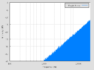
image from en.Wikipedia.org/wiki/Violet_noise#Violet_noise on 12/11/2008
THE REVERSE PROCESS
Knowing how to convert data to a color of noise is only half the problem. What if we know what type of noise is possible and we need data from it for a given process? Knowing the noise color means that we know the power spectral density relation to the frequency. From here onwards we follow the reverse route as that taken to get to the noise color by using the inverse Fourier transform instead.
Inverse Fourier Transform
\[x(t)=\frac{1}{2 \pi} \int_{-\infty}^{\infty} X(w) e^{j w t} d t \nonumber \]
where;
- is the equation of the curve to produce future the data.
 is the exponential form of writing the relation
  . The j in the second term here indicates that that term is imaginary.
- is the frequency
We can either use it to produce a curve or, by making a similar simplification as we did for the Fourier transform, to generate data directly. This reverse process should be trivial to someone who worked through the forward process.
Pops, Snaps & Crackles
The second category of noise is non-frequency based noise. Three examples of this non-frequency noise are pops, snaps and crackles. The study of these noise types is fairly new, and not a lot is known about how to deal with them when they arise in our research or studies. However, one can successfully distinguish and classify these noise types by noticing certain properties which are typical of them.
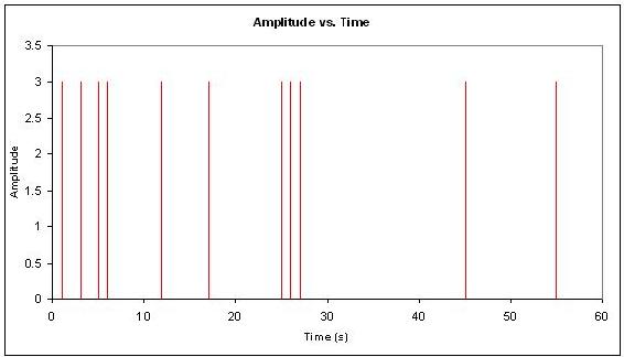
Pops
At one end of the extreme of non-frequency noise is what is defined as pops. Pops are infrequent random spikes in noise of approximately the same amplitude. An example of this would be a loose wire that is usually completing the circuit. However, it randomly disconnects for a split second and then recompletes the circuit for normal operation. Chemical engineering processes may inherently have pops that are unpredictable. Safety features can be added to a process, such as pressure relief valves, to handle the pops when they do occur. The following is an image of what pops might look like in a system:
Snaps
On the other end of the non-frequency noise spectrum there are snaps. Snaps are single independent events that occur only once. When a pencil is bent and it breaks under the force is an example of snapping. Another example would be the snapping of a piece of chalk or exploding a bomb. The “popping” of one’s knuckles is really snapping since it is an independent event, unless you snap all your knuckles all at once or one after the other really fast. Just like pops, snaps are unpredictable, and safety features should be added to the system to handle the snaps. The following is an example of a snap:

Crackles
In between popping and snapping there is crackling. A very common example for crackling is the sound heard coming from a burning piece of wood. Like popping, there is a non-frequency or irregularity in which the crackles occur. In addition, there is also an irregularity of the amplitude of the crackle. In the case of the fire, not only can you not predict when the crackle sound would be heard, but you cannot predict how loud it will be either. Furthermore, there is a universality condition associated with crackling. Regardless of the scale, the similar randomness in repetition and amplitude should be observed.
In dealing with this universality condition the concept of a critical exponent arises. For example, if we are looking at the same crackling effect, \(S\), over a larger period of time the two would have to be equal after scaling the larger one.
\[\langle S \rangle_{\text {small}}(T)=A\langle S \rangle_{\text {large}}\left(\frac{T}{B}\right) \nonumber \]
for some scaling factors  and
and  .
.
where \(\langle S \rangle\) is S average.
If the time scale is expanded by a small factor \(B=\left(\frac{1}{(1-\delta)}\right)\) then the rescaling of the size will also be small, say \(1+a \delta\).
\[\langle S \rangle(T)=(1+a \delta) *\langle S \rangle(1+\delta T) \nonumber \]
For small \(\delta\) we have
\[a\langle S \rangle=T \frac{d\langle S \rangle}{d T} \nonumber \]
Solving gives
\[\langle S \rangle(T)=S_{o} T^{a} \label{eq20} \]
The exponent \(a\) is called the critical exponent and is a universal prediction of a given theory. There are other concepts which are used as a check for universality for times when the critical exponent cannot be used but the most common one is the critical exponent. The following is an example of what a crackle might look like in a system:
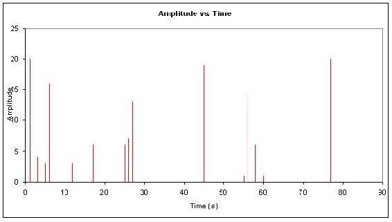
A lead engineer monitoring the instantaneous flow rate of a coolant used to cool an exothermic reactor gathers data set ‘a’ over a 30hr period. Later on that week he gathers data set ‘b’ for the same coolant flow rate. For both sets of data he determined that the way the instantaneous coolant flow rate is reacting to the exothermic reactor is optimal to the reaction process. For his records he would like to represent the noise in the data in a compact form. He wants you to first characterize the noise and then provide any other information, which will generalize the trend in the data. Once you have completed these tasks, report back to him.
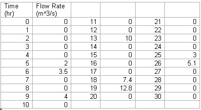
Data set 'a'
Note that between 0 and 30hr for all intervals of time not represented in this table there is a zero assigned as the instantaneous flow rate.
Data set 'b'
Note that between 0 and 50hr for all intervals of time not represented in this table there is a zero assigned as the instantaneous flow rate.
Solution
Each set of data is plotted, Flow Rate vs. Time. The two graphs show crackling trends.
Graph for data set 'a'
Graph for data set 'b'
Upon observing this, the general noise trend is crackling. To provide a final proof we apply the universality relation (Equation \ref{eq20}).
We first determine the critical exponent, \(a\), for data set a.
We see that;
\[<S>=1.54 \nonumber \]
\[\\ S_0 = 2 \nonumber \]this value can be the first value attained or an average of the first 2 or 3 values.
\[T=30\nonumber \]
Solving for the critical exponent using the relation given above we get;
\[a=-0.08\nonumber \]
Once again we carry out the same calculation for data set 'b'.
\[<S>=2.12\nonumber \]
\[\\ S_0 = 3 \nonumber \]this value can be the first value attained or an average of the first 2 or 3 values
\[T=50\nonumber \]
Solving for the critical exponent using the relation given above we get;
\[a=-0.08\nonumber \]
The similarity of the two critical exponent gives further proof that the data the instantaneous flow rate of the coolant over a period of time will show crackling.
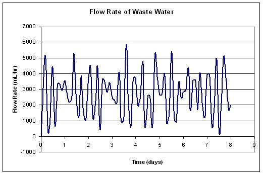
A chemical engineer is reading flow rates from flow meter. Every 0.1 day for 8 days a reading was taken and the data is given here: Colors of Noise Example. The data displays the fluctuations from the set flow rate of 3000 liters per hour at a wastewater treatment plant. The specifications for the plant say that the max flow rate is 6000 liters per hour, or the pipes will burst. Also, the flow rate cannot fall below 200 liters per hour, or the system will automatically shut down.
The chemical engineer notices that there were some readings close to these limits. It is the chemical engineer’s job to determine if the readings are accurate flow rates or if there is an error with the flow meter. By characterizing the type of noise, the chemical engineer can determine the source of the noise and so take appropriate preventative measures. What type of noise is present and what protective measures should be taken?
Solution
1) Plot data. From the data presented, a flow rate vs. time chart was graphed to gauge degree of fluctuation in the flow rate.
2) Calculate the power spectral density data. Using the simplified integral derived to calculate the power spectral density, a table was created with the resulting PSD values at varying frequencies. These frequencies were self defined and were chosen to encompass a broad range. More detailed calculations can be found here: Colors of Noise Example under the worksheet titled “PSD CALC”.
3) Plot the power spectral density. The power spectral density for each frequency was then plotted against the frequency, creating the power spectral density plot shown below.
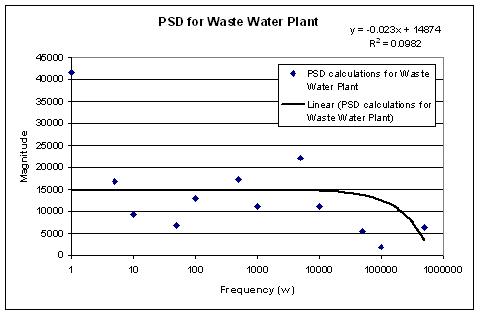
4) Characterize the noise. To determine the β value for the data, a linear trend line was taken on the data. This trend line can be seen in the power spectral density plot above. The slope of this trend line is the β value for the data. In this case, the β=0.023. Since this value is not that of white noise (β=0) nor that of pink noise (β=1), we can say that this noise is somewhere between white and pink noise.
5) Determine the source of noise.
There are two possible major sources of noise. They are the liquid motion in the pipe and noise in the flow meter caused by itself or outside sources. Since it is found earlier that β=0.023, the source of noise is probably from the flow meter. It is not from the motion of liquid in the pipe because liquid motion tends to produce brown noise (β=2).
6) Protective measures that can be taken. Knowing this, a correction can be made on the calculations to determine the actual flow rate. A full step by step solution can also be found here: Colors of Noise Example under the worksheet titled “Solution”.
Summary
Noise is all around us and is an unavoidable characteristic of monitoring signals. When noise is frequency based, like the colors of noise, it can be characterized and modeled using mathematical tools. When noise is not frequency based, like pops, snaps, and crackles, it can be recognized, but ways to model it are still being devised. Characterizing and modeling noise is important for chemical engineers to accurately handle their data, control processes, and predict future trends.
References
- Kosko, Bart. “White Noise Ain’t So White”, Noise. ISBN 0670034959
- Ziemer, Rodger E. Elements of Engineering Probability and Statistics, New Jersey: Prentice Hall. ISBN 0024316202
- Papoulis, Athanasios. Probability, Random Variables, and Stochastic Processes, New York: McGraw – Hill Book Company. ISBN 0071199810
- Peebles, Peyton Z. Jr. Probability, Random Variables, and Random Signal Principles, New York: McGraw – Hill, Inc. ISBN 0071181814
- Sethna, James P. Crackling Noise, Nature 410, 242-250 (2001). Also available here.
- en.Wikipedia.org
Contributors and Attributions
- Authors: Danesh Deonarain, Georgina Mang, Teresa Misiti, Carolyn Ehrenberger
- Date Presented: September 08, 2006 Date Revised: September 19, 2006