
2.9: Helpful Mathematica Syntax- Hints on how to use Mathematica to model chemical processes
- Page ID
- 22372

Section 9. Helpful Mathematica Syntax: Hints on how to use Mathematica to model chemical processes
Title: Useful functions in Mathematica as pertaining to Process controls
Introduction
Mathematica has many different functions that are very useful for controlling chemical engineering processes. The Mathematica syntax of these functions is often very complicated and confusing. One important resource is the Mathematica Documentation center, which is accessed through the program help menu. The Documentation Center provides an extensive guide of every function in the program including syntax and sample code. A "First Five Minutes with Mathematica" tutorial is also present in the menu, which provides a quick guide to get started with Mathematica. This article will briefly outline several useful Mathematica functions and their syntax.
Mathematica Basics
Here are some basic rules for Mathematica.
Notebook, Cells and Evaluation
The standard file for Mathematica is called a notebook. The notebook consists of two kinds of cells: input and output. The inputs are typed into one cell and the outputs are displayed in another (See Below).
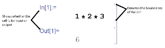
In order to have Mathematica calculate your inputs, you must evaluate the cells. Do this by pressing Shift+Enter. This will only evaluate the current cell that your cursor is located. To evaluate all the cells of a notebook press Ctrl+A, to select all, and then press Shift+Enter.
Parentheses vs. Brackets
Brackets, [], are used for all functions in Mathematica. The only thing parentheses, (), are used for is to indicate the order of operations.
Equality, = vs. ==
The single equal sign (=), is used to assign a value or a function to a variable. The double equal sign (==) is used to set two values equal to each other, such as solving for a value, or to test equalities. When testing equalities, Mathematica will output 'True' or 'False.'
If you recieve 'True' or 'False' as an output when you are expecting it, you likely used a == somewhere that you should have used a =.
Semicolon Use
Placing a semicolon after a line of code will evaluate the expression; however, there will be no output shown.
Mathematica Functions
All Mathematica functions start with a capital letter, eg. Sin[x], Exp[x], Pi or Infinity.
Assigning and Inserting Variables or Parameters
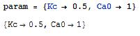
To assign values to variables, use -> rather than an equals sign. For example,
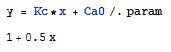
To insert a set of parameters to a function use /. This symbol applies a rule or list of rules in an attempt to transform each subpart of an expression.
For example, if you want to enter the above parameters into the expression y = Kc * x + Ca0, enter the following in Mathematica:
Variables are case sensitive. For example, X is different than x. Also, if you define a variable, it will remain defined until you redefine it as something else or clear it. You can clear a variable, for example, x, by using the Clear[x] command. You can also quit the Kernel, which will clear all variables.
Forcing a Numerical Expression
To force Mathematica into giving a numerical solution, use the function N[expression]. For example,
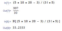
Another method to do this is to place a decimal place in any of your numbers (i.e. "5." instead of just "5")
Integration
Mathematica can do some very complex integrations with fairly little coding. Integration can be very helpful for many engineering applications, but when the functions become very complex they become increasingly difficult to integrate. Mathematica will integrate any function that is possible to integrate.
To integrate a function f(x) the Mathematica, the command is Integrate[].
For an indefinite integral the correct coding is Integrate[f(x),x] where x is the independent variable.
For a definite integral with limits of y and z the correct coding is Integrate[f(x),{x,y,z}]
For example:
We can integrate a function like the one below:
f(x) = Sin(5 * x / 8) * x
We can find the indefinite integral as seen here:
We can find the definite integral from 0 to π as seen here:
Solver
Mathematica's Solve function attempts to solve an equation or set of equations for the specified variables. The general syntax is Solve[eqns, vars]
Equations are given in the form of left hand side == right hand side.
A single variable or a list of variables can be also be specified. When there are several variables, the solution is given in terms of a list of rules. For example,
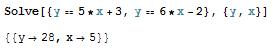
When there are several solutions, Solve gives a list of them. For example,
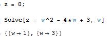
Solve will not always be able to get explicit solutions to equations. It will give the explicit solution if it can, then give a symbolic representation of the remaining solutions in terms of root objects. If there are few symbolic parameters, you can the use NSolve to get numerical approximations to the solutions.
Plotting
Mathematica contains a very powerful plotting interface and this overview will go over the basics of plotting. Using Mathematica's Plot[ ] function there is a basic syntax to be used:
Plot[function, {variable, variable_min, variable_max}]
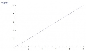
For example, the command "Plot[y=x, {x,0,10}]" will output a graph of the function y=x for a range of x from 0 to 10.
The function could also be previously defined and then referenced in the Plot [ ] command, this functionality provides a lot of simplicity when referencing multiple functions and helps prevent a typo from affecting your Plots.
y[x]==x
Plot[y[x],{x,0,10}]
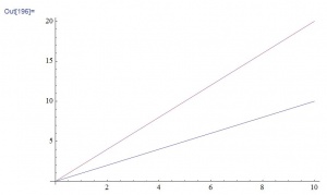
To plot multiple functions on the same plot, use an array of functions using curly brackets { }, in place of the single one:
Plot[{y=x,y=2*x}, {x,0,10}]
Another useful plotting option in Mathematica is the ListPlot function. To use this function, the following formatting should be used: ListPlot[Table[f(x),{x,min,max}] 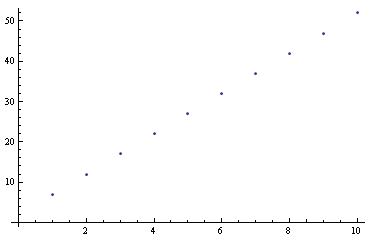
This is obviously only the basics, Mathematica provides many more options including colors, legends, line styles, etc. All of these extra features are well documented at Wolfram's Reference Site.
An additional piece of information: Type the following command on the line after the Plot command to determine the max value plotted. It will display the number associated with the absolute max of the function within the plotting range.
Max[Last/@Level[Cases[%,_Line,Infinity],{-2}]]
Solving ODEs
Within Mathematica, you have the option of solving ODEs numerically or by having Mathematica plot the solution.
Explicit solution:
The built-in function DSolve solves a differential equation or a list of differential equations for either one indepedent variable or a list of independent variables, which solves a partial differential equation. The most basic syntax for the function DSolve is DSolve[eqn,y,x]. For example,
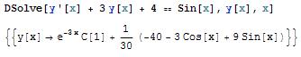
The syntax for solving a list of differential equations is DSolve[{eqn1,eqn2,...},{y1,y2,...},x], while the syntax for solving a partial differential equation is DSolve[{eqn, y, {x1,x2,...}]. For example,
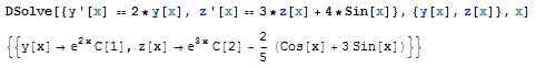
Note that differential equations must be stated in terms of derivatives, such as y'[x]. Boundary conditions can also be specified by giving them as equations, such as y'[0]==b.
Plotted Solution:
Solutions given by DSolve sometimes include integrals that cannot be carried out explicitly, thus NDSolve should be used. NDSolve finds a numerical solution to an ordinary differential equation within a specified range of the independent variable. The result will be given in terms of InterpolatingFunction objects, and thus the solution should be plotted. For example,
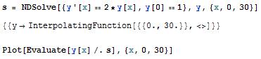
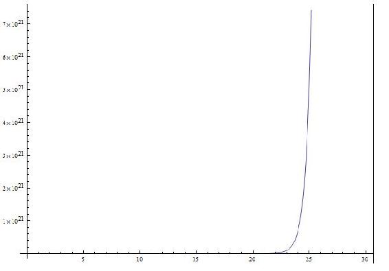
Note that a place holder was defined to store the NDSolve solution in order for the solution to be plotted. The general syntax for plotting is Plot[Evaluate[y[x] /. s], {x, xmin, xmax}], where s is said placeholder. The plot below shows the solution to this example.
Another Example Solving ODEs
In this example the water level of a tank is controlled by adjusting the feed rate of water into the tank. The system is modeled by the following equation:
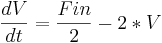
There is a PID controller on the valve but is not important in explaining the Mathematica syntax. Consider it just a different way to define Fin.
Parameters are assumed to be Vset = 10, Kc = 10, tauI = 0.1, and tauD = 1
For this problem the differential equation needs to be modeled with the given parameters in Mathematica. The problem asks what the steady state of the system is. This is solved for by substituting in a PID expression for Fin (not important in this context), setting the derivatives equal to zero, and solving for V and Xi(a made up variable for the PID controller). The following Mathematica code does all said things.
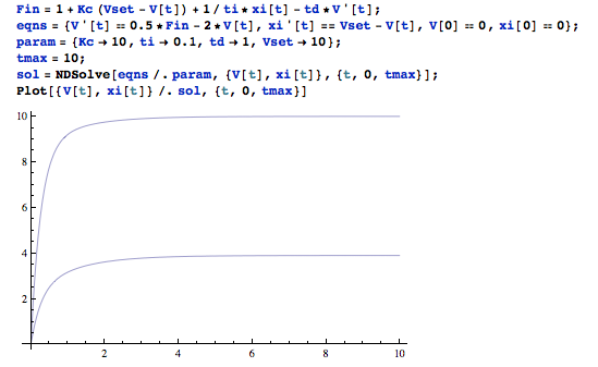
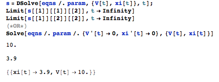
The final line shows that the steady state values for the problem are V = Vset or 10 units of volume, and Xi (the made up variable for the PID controller) has a steady state value of 3.9
In this example there is syntax for defining parameters, applying those parameters to equations, setting up equations, and solving equations for steady state values. There is also syntax for plotting multiple equations on the same graph and how to evaluate multiple functions over time periods. Overall very useful for solving Controls Engineering problems in Mathematica.
Matrix
It is very simple to create a matrix in Mathematica. Simply pick a name for the matrix (for this example we will use a) then simply enter each row inside of curly brackets {} with the individual values separated by commas, and the the row separated by a comma. The function MatrixForm[] will display a matrix in its matrix form rather than as a list of numbers.
EX: a =
Callstack:
    at (Bookshelves/Industrial_and_Systems_Engineering/Chemical_Process_Dynamics_and_Controls_(Woolf)/02:_Modeling_Basics/2.09:_Helpful_Mathematica_Syntax-_Hints_on_how_to_use_Mathematica_to_model_chemical_processes), /content/body/div/div[8]/p[2]/span, line 1, column 2
MatrixForm[a] displays:
5 2 3
7 9 11
8 13 9
You can refer to any specific position in the matrix by using the system:
matrix[[row],[column]]
EX: For the matrix above a[[1],[2]] a value of 2 would be returned.
Jacobians and Eigenvalues
The Jacobian is a helpful intermediate tool used to linearize systems of ODEs. Eigenvalues can be used with the Jacobian to evaluate the stability of the system. Mathematica can be used to compute the Jacobian and Eigenvalues of a system by the following steps.
1. Enter the system as individual equations
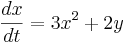
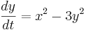
entered as
eq1 = 3*x^2+2y
eq2 = x^2-3*y^2
2. Compute the Jacobian with Mathematica's Derivate function
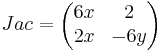
computed by
Jac =
Callstack:
    at (Bookshelves/Industrial_and_Systems_Engineering/Chemical_Process_Dynamics_and_Controls_(Woolf)/02:_Modeling_Basics/2.09:_Helpful_Mathematica_Syntax-_Hints_on_how_to_use_Mathematica_to_model_chemical_processes), /content/body/div/div[9]/p[11]/span, line 1, column 6
3. Use Mathematica's Eigenvalues function to evaluate the stability of the system
Begin by entering a desired value of {x,y} into the matrix (i.e. steady state values of x and y).
Jac = 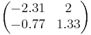
Then call the Eigenvalue function.
Eigenvalues[Jac]
Result: λ={-1.82, 0.85}
The Jacobian can be computed as long as the matrix is square. Many other function types are acceptable when entering eq1 and eq2, including trigonometric and exponential functions.
User-Defined Functions
Mathematica also supports user-defined functions. Defining your own functions helps to simplify code, especially when lengthy expressions are used consistently throughout the code. The generic Mathematica syntax for defining a function is as follows:
f[a_,b_,c_]:=(a+b)/c
Here, the function name is "f" with three arguments: a, b, and c. The syntax ":=" assigns the expression on the right hand side to the function "f." Make sure that each of the arguments in the brackets on the left hand side are followed by underscores; this identifies the variables being called by the function as local variables (ones that are only used by the function itself). For this example, the function "f" will take three arguments (a, b, and c) and calculate the sum of a and b, and then divide by c.
After defining the function, you can use the function throughout your code using either real numbers, as the first example shows, or any variables. This is done by calling the function with the correct number of arguments. When referencing variables, if the variable already has an assigned value the value will be used, if it does not, Mathematica will display your function's results with the variables displayed. A few examples are shown below.
![[1,3,2]=\frac{1+3}{2}=2](https://eng.libretexts.org/@api/deki/files/17182/image-174.png?revision=1)
![[x,y,z]=\frac{x+y}{z}](https://eng.libretexts.org/@api/deki/files/17184/image-175.png?revision=1)
Nonlinear Regression
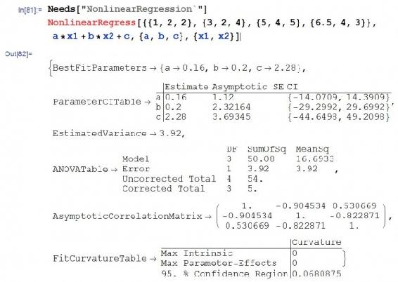
Mathematica can be used to solve multiple variable, nonlinear regression problems. This form of regression can be useful to create models of how temperature or pressure sensors depend on different valves in a system. The NonLinearRegress function in Mathematica can be used to find a best-fit solution to a user defined functional form.
The NonLinearRegress function is not part of the standard package in Mathematica. For this reason, this function must be loaded into Mathematica before an attempt to use.
After this step, the NonlinearRegress is loaded and can be used to solve for a set of data. To use the this function, enter NonlinearRegress[data, expression, parameters, variables]. The best fit values for the parameters will be returned along with statistical information about how well this form fits the given data. An example of Nonlinear Regression in Mathematica is shown in the image below.
Probability Density Function
Often in controls, it is necessary to calculate the probability that a certain event will occur, given a particular known distribution. In these scenarios, it is helpful to know how to use the built-in probability density function in Mathematica. The syntax for using the probability density function to calculate the probability of observing a value x for a generic distribution dist is shown below.
PDF[dist,x]
A variety of distributions can be used in conjunction with the probability density function. These distributions include the normal distribution and the binomial distribution.
Normal Distribution
For a normal distribution with a mean μ and a standard deviation σ, use the following syntax to specify the distribution.
NormalDistribution[μ,σ]
To calculate the probability of observing a value x given this distribution, use the probability density function as described previously.
PDF[NormalDistribution[μ,σ],x]
To calculate the probability of observing a range of values from x1 to x2 given this distribution, use the following syntax.
NIntegrate[PDF[NormalDistribution[μ,σ],x],{x,x1,x2]
For the theory behind the probability density function for a normal distribution, click here.
Binomial Distribution
For a binomial distribution with a number of trials n and a success probability p, use the following syntax to specify the distribution.
BinomialDistribution[n,p]
To calculate the probability of observing a successful trial exactly k times given this distribution, use the probability density function as described previously.
PDF[BinomialDistribution[n,p],k]
To calculate the probability of observing between a range of k1 number of successes and k2 number of successes given this distribution, use the following syntax.
NIntegrate[PDF[BinomialDistribution[n,p],k],{k,k1,k2]
Alternatively, binomial distribution can be found using a user defined function. Define the equations as follow: binom[nn_,kk_,pp_]:= nn!/(kk! (nn-kk)!) pp^kk (1-p)^(nn-kk)
where:
number of independent samples = nn
number of events = kk
probability of the event = pp
To find the odds of getting 5 heads out of 10 coin tosses,assuming the probability of head = 0.5, substitute the values for nn,kk and pp as following: binom[10,5,0.5]
Using the same scenario, but instead for the odds of getting 5 or more heads in the 10 tosses, the function can be used as: Sum[binom[10,i,0.5],{i,5,10}]
For the theory behind the probability density function for a binomial distribution, click here.
Manipulate Function
Often in controls, it is useful to manipulate certain variables dynamically and see the result in a plot or table. This is particularly useful in setting the constants in tuning PID controllers. The Manipulate function in Mathematica lets you do this. You can use the manipulate function in conjunction with the Plot command. The general syntax for using the manipulate function is as follows:
Manipulate[expr,{u,umin,umax}]
Where expr is the function that you want to add controls to and u is the variable you wish to manipulate.
Manipulate a function:
You can change the variable x in the function s. Moving the bar lets you change the variable x.

Manipulate a plot:
You can also manipulate a plot. The slider bar lets change the variable n and the plot changes accordingly.

The Mathematica file used to create this example, can be downloaded below.
Manipulate Command Example
For more information regarding manipulate, please see the Wolfram's Reference Site.
[Note - need to add manipulate for the Bode plots - R.Z.]
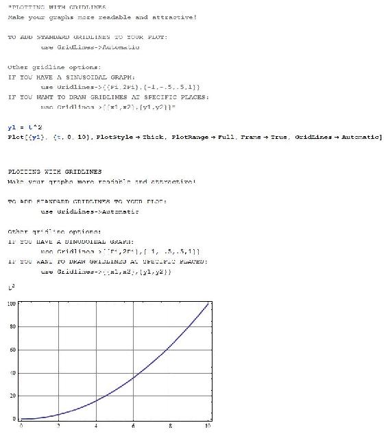
Adding Gridlines
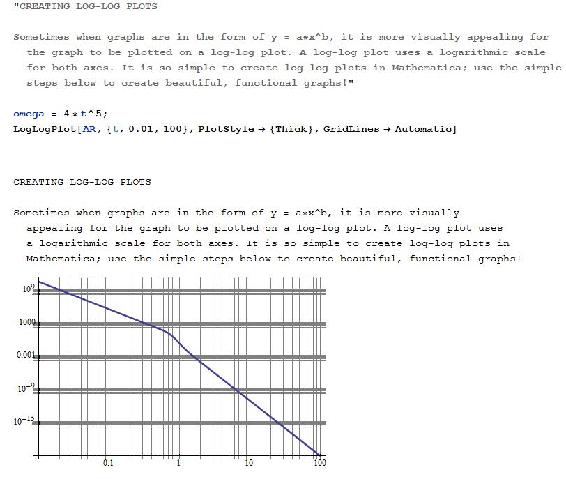
Plotting Log-Log Graphs
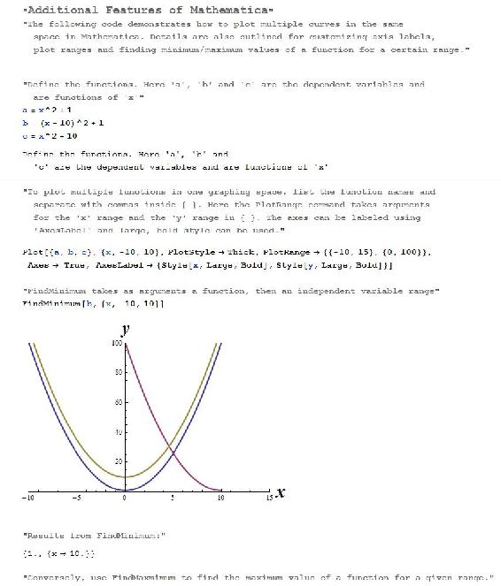
Other Useful Mathematica Tips
[It would be good to replace this images with actual text - R.Z.]