2.4: Excel Modeling - logical models, optimization with solver for nonlinear regression, sampling random numbers

Introduction

Microsoft Excel program is one of the most popular and useful computer programs for a wide variety of numerical applications. Excel features several different functions, interfaces and graphing tools which can be applied in many fields. The following functions might be especially useful for logical programming in Excel:

• Logical functions (ex: IF, OR and AND): These functions can be used in control analysis, particularly in safety regulation (for example, if the temperature exceeds X degrees, shut down the reactor and send cooling water to the jacket)
• Solver: This function can be used to maximize, minimize or try to obtain an input value in a cell by varying referenced cells.
• Random Number Generator. This can be used as a tool for probability or randomly selecting data points for analysis from a large pool of points.

While it might be less accurate than other modeling programs, the Excel model provides good estimates, and facilitates observation and understanding of process behavior while requiring minimum computer knowledge. The following sections will provide you with a better understanding of these common Excel functions, followed by examples in engineering applications.

Logical Methods

A logical test is any expression that can be evaluated as TRUE or FALSE with specified input conditions. Commonly used logical tests are IF, OR and AND statements. All three statements can be used in conjunction with each other for more complex and complete modeling.

Note: all functions and formulas in Excel require an equal (=) sign in front of the syntax.

Excel's IF statement

The IF function in Excel tests values and formulas in the target cells and returns one specified value "if" the condition input evaluates to be TRUE and another value if it evaluates to be FALSE. The IF statement in Excel is called out with the following syntax:

• IF(logical_test,value_if_true,value_if_false)

Logical_test: any expression or correlation of values that can be evaluated as TRUE or FALSE.

Value_if_true: the value or expression that is returned IF the condition in the logical test returns TRUE.

Value_if_false: the value or expression that is returned IF the condition in the logical test returns FALSE.

The value_if_true and the value_if_false part in the syntax may vary and can be numerical values, expressions, models, and formulas. If either of the values is left blank, the test will return 0 (zero) correspondingly.

Sample coding:

• IF(1+1=2, "Correct!", "Incorrect!")

For the logical test part, 1+1 is equal to 2, and the iteration will return TRUE. The value_if_true is called for the TRUE response, and "Correct!" will be output in the corresponding cell.

It is possible to nest multiple IF functions (called Nested IF) within one Excel formula. Such a formula is useful in returning multiple answers, compared to a a single IF function which can return only two possible answers.

A Nested IF statement has the following syntax:

• IF( logical_test1, value_if_true1, IF(logical_test2, value_if_true2, value_if_false) )

The following example shows how a Nested IF function is used to make a spreadsheet that assigns a letter grade to different scores.

Suppose that grade distribution is:

@ A= Greater than or equal to 80

@ B= Greater than or equal to 60, but less than 80

@ C= Less than 60

This logic function can be written in several different ways. If the score is tested to be the letter grade C first, then checked to see if it is a B or an A, the syntax could be written as follows:

• IF(A5<60,"C",IF(A5<80,"B","A"))

Note that the Nested IF statement can be placed in either the value_if_false OR the value_if_true positions. In the example above, it was placed in the value_if_false position because of how the conditional was written.

Additional letter grades could be added by including more nested IF functions inside the existing function. One formula can include up to 7 nested IFs, which means you can return up to 8 different results.

Excel's OR statement

The OR statement in Excel is similar to the IF statement. It returns TRUE if any argument or expression of values is TRUE, and it returns FALSE if all arguments or expression of values are FALSE. The syntax for OR is:

• OR(logical1,logical2,...)

logical1: there can be up to 30 arguments for the logical expression to test and return either TRUE or FALSE. If all of the arguments are false, the statement returns FALSE for the entire expression.

Sample coding:

• OR(1+1=2, 2+2=5)

In the logical1 part, 1+1 is equal to 2 and will return TRUE. In the logical2 part, 2+2 is not equal to 5 and will return FALSE. However, since one of the test returns TRUE (logical1), the function returns TRUE even if logical2 is FALSE. TRUE will be output in the corresponding function cell.

Excel's AND statement

The AND statement returns TRUE if all its arguments or values are TRUE and returns FALSE if one or more argument or value is FALSE. The AND statement syntax is:

• AND(logical1,logical2,...)

logical1: similar to OR statement with up to 30 arguments to test that could return either TRUE or FALSE.

Sample coding:

• AND(1+1=2, 2+2=5)

Logical1 will return TRUE for the correct calculation while logical2 will return FALSE for the incorrect calculation. However, since one of the expressions is FALSE, the AND logical test will return FALSE even if one of the tests is true.

It is common and useful to understand how to implement different logical functions into each other. A good example would be:

• IF(AND(2+2=4,3+3=5),"Right Calculation","Wrong Calculation")

During iteration, the AND statement should return FALSE since one of the expression/calculation is incorrect. The FALSE return will output "Wrong Calculation" for the IF statement iteration.

Other Useful Excel Functions

Excel has many useful functions that can help any engineer who is using Excel to model or control a system. An engineer may want to know the average flow rate, number of times the liquid in a tank reaches a certain level, or maybe the number of time steps that a valve is completely open or completely closed. All of these situations and many more can be addressed by many of the simple built-in functions of Excel. Below are some of these functions and a brief definition of what they compute and how to use them. They are followed by an image of a sample excel file with an example of each function in use. To see a list of all the built-in functions Excel has to offer, click shift-enter on the cell.

AVERAGE(number1,number2,...) - Returns the average or arithmetic mean of the arguments. The arguments can be numbers, arrays, or references that contain numbers.

CEILING(number1, significance) - Rounds a number up to the nearest integer or multiple of significance.

CHIDIST(x, degrees_freedom) - Returns the probability of the chi-squared distribution.

COUNT(value1,value2,...) - Counts the number of cells that contains numbers.

COUNTIF(range, criteria) - Counts the number of cells within the range that meet the given criteria.

COUNTIFS(criteria_range1,criteria1,criteria_range2,criteria2,...) - Counts the number of cells within multiple ranges that meet multiple criteria.

FLOOR(number1,significance) - Rounds a number down toward zero, to the nearest multiple of significance.

FREQUENCY(data_array,bins_array) - Calculates how often a value occurs within a range of values (bins). The function will return a vertical array of numbers having one more element than the bins_array. Once the formula is entered into the target cell, highlight the target cell making a vertical array one cell larger than bins_array. Once selected press F2 to open the formula of the target cell and then press CTRL+SHIFT+ENTER to execute your function.

LARGE(array,k) - Returns the k-th largest value in a data set. For example, the 2nd largest number.

MAX(number1,number2,...) - Returns the largest number in a set of values.

MEDIAN(number1,number2,...) - Returns the median of a set of values.

MIN(number1,number2,...) - Returns the minimum value in a set of values.

MODE(number1,number2,...) - Returns the most frequently occurring value in an array or range of values.

PERCENTILE(array,k) - Returns the k-th percentile of values in a range

ROUND(number1, num_digits) - Rounds a number to the specified number of digits.

SMALL(array,k) - Returns the k-th smallest value in a data set. For example, the 7th smallest number.

STDEV(number1,number2,...) - Returns the standard deviation of a given set of values ignoring text and logical values.

SUM(number1,number2,...) - Adds all of the values in a range of cells.

SUMIF(range,criteria,range,...) - Adds values of cells in a range meeting criteria.

VAR(number1,number2,...) - Estimates the variance of a given set of values.

Nesting

Though not complex or difficult, placing logical statements within one another can be a powerful practice. This is referred to as nesting.

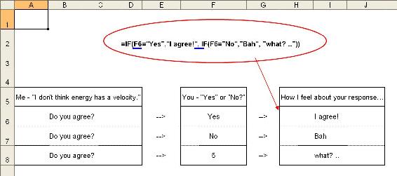
An example demonstrating the use of a simple IF statement nested within another IF statement is shown below:

If one were to ask three individuals whether or not they agree that energy has a velocity, these individual will hypothetically respond in one of three ways: "Yes","No", or (other). In this case, if the individual were to respond "Yes", then the questioner would respond "I agree!". If the individual were to respond "No", the questioner would bitterly respond with a "Bah". And if the individual were to respond with a nonsensical answer, then the questioner would respond "what .." in confusion.

The important point to get out of this example is that nested statements gives us the potential to process more information in one cell (or line of programming code).

Excel's Data Analysis Tools

Excel has several useful built in add-ins that can make data analysis much easier. Of these we will cover the solver tool, as well as the ANOVA analysis.

Solver Tool

The solver in Excel is a built-in tool with multiple capabilities. It could be used to optimize (find the maximum or the minimum value) a specific cell (the target cell) by varying the values in other cells (the adjustable cells). It may also be used to solve a system of non-linear equations. Solver formulas embedded in the spreadsheet tie the value in the target cell to the values in the adjustable cells. The user can also specify numerical range constraints for the cells involved.

Optimization Model

In optimization, one seeks to maximize or minimize the value of a real function. Just as a student in a calculus class might use optimization techniques to find a local maxima or minima of a complex function, a CEO might use similar techniques to find how much product their company should manufacture to maximize profits. There are numerous optimization techniques, many specialized for specific types problems. For the most part, MS Excel uses gradient-based techniques.

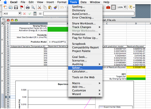
The solver tool is located in the Tools menu. If it does not appear there, it must be added in by selecting Add-ins and selecting the appropriate check box.

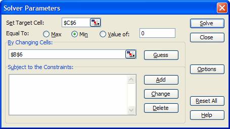
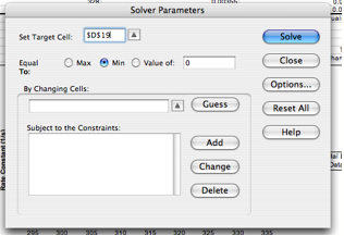
The solver window contains the following fields:

• Set Target Cell: This is the cell containing the value you want to optimize.

• Equal To: Choose whether to maximize the value, minimize the value, or set it to a specific number.
• By Changing Cells: Here you specify all the cells that can be varied when optimizing the target cell value.
• Subject to the Constraints: Constraints are optional, but can be added by clicking Add and defining each constraint.
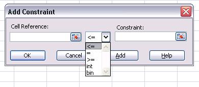
• List of Available Constraints

• <= (Less than or equal to) Stipulates that a selected cell must be less than or equal to a certain value.
• = (Equal to) Stipulates that a selected cell must be equal to a certain value.
• >= (Greater than or equal to) Stipulates that a selected cell must be greater than or equal to a certain value.
• int (Integer) Stipulates that a selected cell must be an integer
• bin (Binary) Stipulates that a selected cell must be equal to 1 or 0.

The window where these constraints can be entered is shown below.

It is important to make sure that constraints do not violate each other otherwise solver will not work without reporting an error. For example, if a cell must be great than 2 and less than 1 Solver will not change anything.

Once all the fields in the Solver window are completed appropriately, click Solve. If solver can find a solution a window will pop up telling you so, and the values will appear in the target and adjustable cells. If solver cannot find a solution it will still display the values it found but will state that it could not find a feasible solution. Be aware that Excel solver is not a powerful enough tool to find a solution to nonlinear equations, where programs such as Matlab might be a better choice.

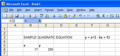
* Guided Example: Suppose you have an Excel spreadsheet set up as shown below, with cell C6 depending on cell B6 according to the quadratic relationship shown, and you want to minimize the value in C6 by varying the value in B6.

1) Open up the solver window.

2) Input C6 in the set target cell field, check the min button, and input B6 in the by changing cells field:

3) Click solve to find the solution.

You can place further constraints or further specify how you want your task solved under "Options." Some of the most commonly used specifications include:

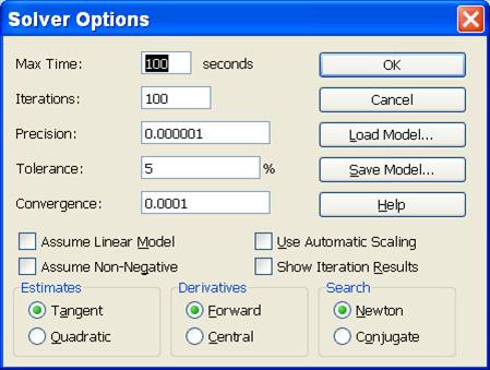
• Max Time: This is the maximum amount of time excel will spend trying to find a converging value before giving up.
• Iterations: This is the number of iterations excel will perform to converge to a value.
• Precision: This is related to how close excel has to get before a value is "acceptable." In general, making this value several orders of magnitude smaller will yield a more accurate result, but will take more time to do so, and may have a harder time converging.
• Tolerance: This is also related to how accurate a solution is, this is related to the percent error. Making this smaller should also yield a more accurate result, but with more difficulty finding a solution.
• Convergence: Controls the amount of relative change that occurs during the last five iterations that Solver performs. The smaller the number of the convergence the less change that will occur.
• Box Options Click on the box to select the following options:
• Assume Linear Model: This will speed up the time to find a solution because it will make Solver assume that the model is linear.
• Assume Non-Negative: Solver will make the lower limit of adjust zero for all the cells that are programmed to be adjusted in the model that are not limited by a chosen constraint.
• Use Automatic Scaling: Used for large differences in magnitude to scale the inputs and outputs.
• Show Iteration Results: Solver will pause between each iteration to show the results of that iteration in the model.
• Estimates Specifies to Solver on how to use initial estimates for iterations
• Tangent: Uses linear extrapolation by utilizing a tanget vector.
• Quadratic: Uses quadratic extrapolation. Best to use for nonlinear models.
• Derivatives Specifies what type of differencing is used for partial derivatives for both the objective and constraints.
• Forward: Constrained values change slowly between iterations.

Nonlinear Regression

Excel's solver function can also be used to find a solution for two-variable non-linear regression. The description of the data by a function is carried out by the process of iterative nonlinear regression. This process minimizes the value of the squared sum of the difference between the actual data and the predicted value (residual).

There are three basic requirements for using solver including:

1. Raw data
2. A model equation to find predicted values
3. Initial guesses for varying values

Before using the solver function, the raw data should be organized into separate columns for the independent variable (first column) and dependent variable (second column). A third column will show the predicted value that is obtained by using the model equation mentioned earlier, and must reference various single cells that have initial values that Excel will use as a starting point for the regression. A fourth column should be created with the square of the difference between the predicted value and the actual experimental value (raw data); this is also known as the square of the residual. A cell at the bottom of this fourth column should include the sum of all the squared difference values above it. Two more cells anywhere else in the worksheet should be designated as the initial guesses for the values to be varied to find the solution.

It is important to choose a reasonable value for the initial guess. This will not increase the chance that Excel arrives at a global optimization rather than a local optimization, but also reduces the time it takes for Excel to solve the system of non-linear equations.

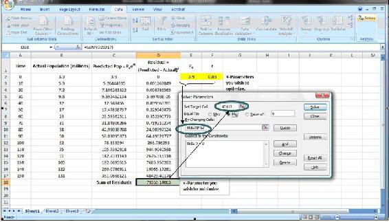
Now, solver can be applied to the spreadsheet to optimize the regression. Refer to section 3.1 for how to access and use solver. The bottom most cell of the fourth column that has the sum of the squares of the residuals will be the target cell. Since the residuals are essentially the error, the sum of the residuals squared should be as small as possible, so the min circle should be selected. The initial guesses should be entered into the "by changing cells". Constraints can be entered if the values of the cells are limited to a certain range. Solver will produce the values of the varying parameters that yield the best fit to the nonlinear data.

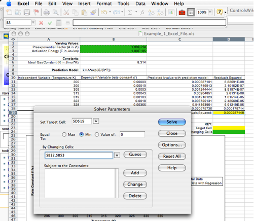
• Guided Example: A screen shot of a simple population problem is shown below. The yellow highlighted cells are the initial guesses for the variables. In this case, the initial population (P0, cell E2) is entered as a constraint.

ANOVA Analysis

ANOVA is another tool on Excel that can be used for data analysis purposes. It is used primarily to compare continuous measurements to determine if they are sampled from the same or different distributions. This is usually done on set of data that consists of numerous samples and/or groups. Single factor ANOVA analyzes the difference between "groups" which can be different units, sensors, etc. On the other hand 2 way ANOVA analyzes the differences on the basis of both samples (trials) and groups, allowing you to compare, which one most affects the system. Two-way ANOVA can be employed for two different cases: data with or data without replicates. Data without replicates is used when collecting a single data point for a specified condition, while data with replicates is used when collecting multiple data points for a specific condition.

The telling result of ANOVA analysis is a p-value telling you if there is a statistically significant difference between data sets. A more in depth discussion of the uses and implementation of ANOVA can be seen here.[1]

Random Number Sampling

A useful numerical technique is the random number generator. This generator uses random number sampling to create a predictive model. This can be especially useful in probability problems.

A typical random number generator produces any number between 0 and 1 with equal frequency. At each step a random number is generated that picks a possible outcome. A typical Excel statement would appear as the following: IF (RAND()<X, value1, value2). This means that X percent of the time, you would get a value1 and 1-X percent of the time, you would get a value2. For example, suppose a situation exists with two possible outcomes, A and B, where A takes place 70% of the time. If a random number is generated that is greater than 0.3, then the outcome is A. Inversely if the random number is less than or equal to 0.3, then B is the outcome. This would be represented as IF(RAND()<0.7, A, B). Each step within the generator does not affect the next step, i.e. each step is determined individually. A process in which previous outcomes do not affect later outcomes is known as a Stochastic method or "Monte Carlo" method. A Monte Carlo simulation uses a model that takes random input that follows an assumed distribution (in this case, 70% A and 30% B) and produces output that models some phenomenon. The following is a simple example of such a simulation:

The Excel is equipped with a random number generator which can be called out using the RAND function. A random number between 0 and 1 can be generated in a cell by the following command:

In Microsoft Excel 2007 the RAND function returns a new random number every time the worksheet is calculated or when F9 is pressed. If the same random number is needed to be referred to more than once in an Excel IF, AND, OR statement, one can create a column of random numbers using =RAND(), and refer back to these cells in an adjacent column.

There are many ways to manipulate the random numbers that Excel produces. A random number can be generated within a different range by multiplying the RAND function by a constant, i.e. multiply by 100 to change a decimal to percent. Another option to generate numbers within a different range is the RANDBETWEEN function. RANDBETWEEN generates a random integer within a specified range. The following command generates a random integer between -6 and 21:

It is also possible to modify your random numbers by nesting the RAND function within another function. For example, one can square the results of one distribution to create a different distribution of numbers.

Another way to utilize the RAND function is to take a random sampling of a data set. If one has a spreadsheet with several hundred data points, and would like to analyze only 100 random points, another column can be created titled "Random Number" or something similar. In the first cell of this column, type the =RAND() function. Then drag this function all the way to the end of the data set. At this point, the user can go to the DATA drag-down menu and select Sort... In this menu, select your random number column in the SORT BY drag down menu. Either ascending or descending can be selected, as desired. Once the spreadsheet is sorted by the random numbered cells, the first 100 data points can be used as a statistically random cross-section of the data.

The sort tool can be useful in cases when you are trying to find out the probability of having certain values above a certain threshold. For example, if the 100 data points that you have represent the temperature variations occurring within a system, you can use sort tool to determine how many temperature values exceed your threshold. From that, you can calculate approximately the probability of the system temperature exceeding the threshold. Two screenshots of the sort process are shown below. Microsoft Excel 2007 uses a different menu, allowing for one to choose between sorting from Largest to Smallest or vice versa. A screenshot below shows this new menu.

Sorting Setup: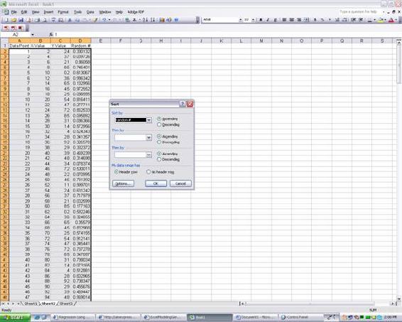

Results to Randomization: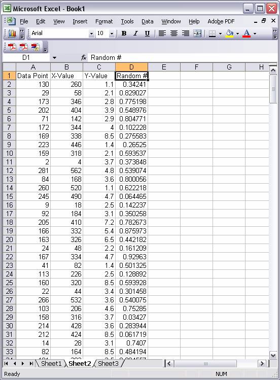

Microsoft Excel 2007: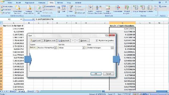

Worked out Example 1

The Arrhenius equation defines the relationship between a reaction rate constant k and temperature:

\[k(T)=A e^{-E / R T} \nonumber \]

where T is the absolute temperature, A is the frequency factor, E is the activation energy, and R is the universal gas constant.

It is frequently desirable to be able to predict reaction rates at a given temperature, but first you need to know the values of A and E. One way to obtain these values is to determine the reaction rate constant at a few temperatures and then perform a nonlinear regression to fit the data to the Arrhenius equation. Given the following rate constant data for the decomposition of benzene diazonium chloride, determine the frequency factor and activation energy for the reaction.

\[\\ (\mbox{s}^{-1}) \nonumber \]	\[\\ (\mbox{K}) \nonumber \]
0.00043	313.0
0.00103	319.0
0.00180	323.0
0.00355	328.0
0.00717	333.0

Solution: The following Excel file contains a solution to the problem that uses Excel's solver tool to perform the nonlinear regression and determine the values of A and E:

Example 1

The spreadsheet is set up as described in the nonlinear regression section above.

1. Open solver (Tools / Solver)

2. Set the Sum of Residuals Squared value cell as the target cell

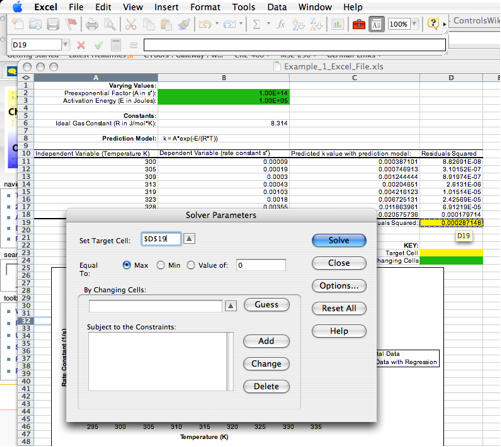
3. Click the Min radio button

4. Set Pre-exponential Factor and Activation Energy as the adjustable cells. For this problem, keep A between 1E+13 and 1E+14 s^-1 and E between 9.5E+4 and 1.05E+5 J

5. Sometimes, depending on what version of excel you are using, a message will come up like the one below. If this happens, click OK. The graph will update with the new curves.

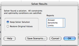
6. Click Solve and observe the values of A and E calculated by Solver and the changes to the plot showing the rate constant as a function of temperature.

NOTE: If solver is not fitting the data well, click the options button in the solver window and make the precision value smaller by several orders of magnitude.

Worked out Example 2

Kinetics can be used to determine the probability of a reaction taking place between gas-phase molecules. Consider molecules A and B, which have a 60% chance of reacting upon collision. Create an Excel spreadsheet that utilizes a random number generator and an if-statement to model an individual collision.

Solution

In this Excel file, sample coding for Random number generator and if-statement is shown.

Collision_ex

Random number generator is used to output numbers between 0 and 1 for four trials, ten trials, and one hundred trials on sheets one, two, and three, respectively. Formula for the random number generator is employed in the cell where you want the number to be output (in this case, B6 is the cell). An IF logical test is then employed to test whether the number follows the requirement or not. The IF-statement cell will then output the corresponding result based on the logic test. In this collision case, if the random number function generated a number greater than 0.4, the logic test will return TRUE and then output "Reacts" as the result. Assuming that the random number generator produces an even distribution between 0 and 1, the random number will be greater than 0.4 sixty percent of the time. Coding of the IF-statement is shown:

On the other hand, if the number generated is less than 0.4, the logic test returns FALSE and "Does not React" will be shown as the result. Different numbers are generated each time the spreadsheet is updated, thus different result will return for the IF function. You can also modify the numbers and return statement to better understand the operation of the functions.

The number of reactions is summed up and divided by the total number of trials to compare the predicted reaction probability with the value given in the problem. It can be seen by comparing sheets one, two, and three that increasing the number of trials decreases the variation in the predicted reaction probability.

Accessing Excel Tools on Windows

On many computers, excel tools such as solver and the data analysis package are not already included and must be installed before used. This section will go over how to access these add-ins for those using Windows opposed to Macs.

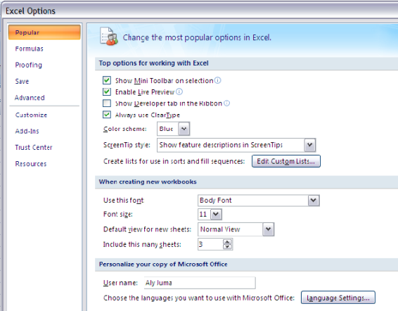
1) Click on the windows symbol in Excel 2007. At the bottom of the opened window, select the Excel options box.

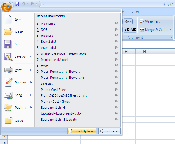
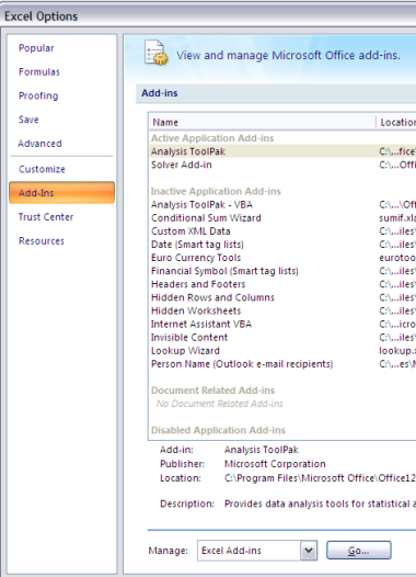
2) On the left side panel you will see a section labeled "Add-ins". Select this.

3) Here you will see a list of "Inactive Applications" that are available for excel. Of these the ones we are interested in are the "Solver Add-In" and the "Analysis ToolPak." Select one of these and click "Go" at the bottom of the window.

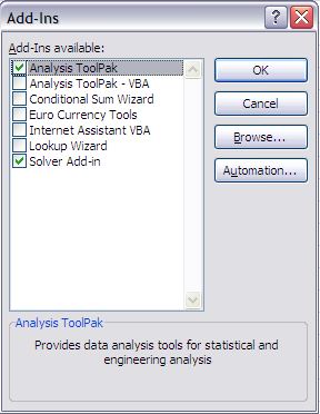
4) A new window will appear asking you which components of the package you would like to install. Select the needed tools (solver and analysis toolpak). Click "Ok" and windows should install the corresponding tools into excel.

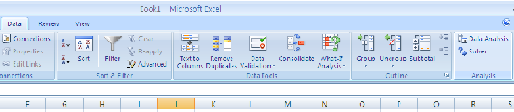
5) Once done, these tools will be found under the data section of Excel, on the far right of the window.

References

1. =RAND()

• =RANDBETWEEEN(-6,21)
• Collision Example Excel File:
• =IF(B6>=0.4,"Reacts","Does not React")
• Bender, E.A. An Introduction to Mathematical Modeling, Mineola, NY: Dover Publications, Inc.
• Fogler, H.S. (2006). Elements of Chemical Reaction Engineering, Upper Saddle River, NJ: Prentice Hall Professional Technical Reference. ISBN 0-13-047394-4
• Microsoft, Excel, Proprietary EULA, www.microsoft.com.

Contributors and Attributions

Authors: (12 September 2006 / Date Revised: 19 September 2006) Curt Longcore, Ben Van Kuiken, Jeffrey Carey, Angela Yeung

Stewards: (13 September 2007) So Hyun Ahn, Kyle Goszyk, Michael Peterson, Samuel Seo