6.9: Blood Glucose Control in Diabetic Patients

Last updated
Save as PDF

Page ID: 22399

$ \newcommand{\vecs}[1]{\overset { \scriptstyle \rightharpoonup} {\mathbf{#1}} } $ $ \newcommand{\vecd}[1]{\overset{-\!-\!\rightharpoonup}{\vphantom{a}\smash {#1}}} $$\newcommand{\id}{\mathrm{id}}$ $ \newcommand{\Span}{\mathrm{span}}$ $ \newcommand{\kernel}{\mathrm{null}\,}$ $ \newcommand{\range}{\mathrm{range}\,}$ $ \newcommand{\RealPart}{\mathrm{Re}}$ $ \newcommand{\ImaginaryPart}{\mathrm{Im}}$ $ \newcommand{\Argument}{\mathrm{Arg}}$ $ \newcommand{\norm}[1]{\| #1 \|}$ $ \newcommand{\inner}[2]{\langle #1, #2 \rangle}$ $ \newcommand{\Span}{\mathrm{span}}$ $\newcommand{\id}{\mathrm{id}}$ $ \newcommand{\Span}{\mathrm{span}}$ $ \newcommand{\kernel}{\mathrm{null}\,}$ $ \newcommand{\range}{\mathrm{range}\,}$ $ \newcommand{\RealPart}{\mathrm{Re}}$ $ \newcommand{\ImaginaryPart}{\mathrm{Im}}$ $ \newcommand{\Argument}{\mathrm{Arg}}$ $ \newcommand{\norm}[1]{\| #1 \|}$ $ \newcommand{\inner}[2]{\langle #1, #2 \rangle}$ $ \newcommand{\Span}{\mathrm{span}}$$\newcommand{\AA}{\unicode[.8,0]{x212B}}$

Background of why insulin control is important for diabetic patients

Diabetes mellitus is a disease of the endocrine system where the body cannot control blood glucose levels. There are two general classifications of diabetes:

Type I (also known as juvenile diabetes)

Genetic predisposition and/or an autoimmune attack destroys T-cells of pancreas
Body cannot produce insulin to regulate blood glucose

Type II

Most common form of diabetes and has reached epidemic status in the United States
Usually caused by lifestyle
Obesity reduces body's responsiveness to insulin

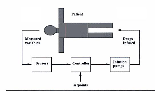
Treatment for both types of diabetes may include exercise, dieting, oral medications, or insulin injections. Most insulin dependent diabetics follow a management plan that requires frequent testing of blood glucose levels and then injection of a prescribed dose of insulin based on the blood glucose level. However, the downside of this treatment method is that there is no predictive control. If blood glucose levels are falling and insulin is administered, a hypoglycemic episode may occur. Recent biomedical advancements have resulted in continuous blood glucose monitoring devices as well as insulin pumps. Continuous monitoring allows for finer blood glucose control and can help predict fluctuations in the blood glucose level. Insulin pumps replace the need to administer insulin injections by automatically injecting a prescribed dose, however it requires blood glucose level input from the patient. In the future, insulin pumps and continuous blood glucose monitors may be integrated forming a closed loop control system which will can replace the body's own faulty control system.

Figure 1: Control Schematic of Insulin Infusion

Mathematical model for a closed loop insulin delivery system

The following set of differential equations are known as the Bergman "minimal model":

\[\frac{d G}{d t}=-p_{1} G-X\left(G-G_{b}\right)+\frac{G_{m e a l}}{V_{1}} \nonumber \]

\[\frac{d X}{d t}=-p_{2} X+p_{3} I \nonumber \]

\[\frac{d I}{d t}=-n\left(I+I_{b}\right)+\frac{U}{V_{1}} \nonumber \]

where:

G = deviation variable for blood glucose concentration
X = deviation variable for insulin concentration in a "remote" compartment
I = deviation variable for blood insulin concentration
G_meal = a meal disturbance input in glucose
U = the manipulation insulin infusion rate
G_b = steady state value of blood glucose concentration
I_b = steady state value of blood insulin concentration

Blood parameters include p₁, p₂, p₃, n, V₁(blood volume). These are specific to the blood specimen and must be predetermined.

A linear state space model can be used to express the Bergman equations seen above. The general form for a state space model can be seen below:

\[\left[\begin{array}{c}
\dot{x}_{1} \\
\vdots \\
\dot{x}_{n}
\end{array}\right]=\left[\begin{array}{ccc}
a_{11} & \cdots & a_{1 n} \\
\vdots & \ddots & \vdots \\
a_{n 1} & \cdots & a_{n n}
\end{array}\right]\left[\begin{array}{c}
x_{1} \\
\vdots \\
x_{n}
\end{array}\right]+\left[\begin{array}{ccc}
b_{11} & \cdots & b_{1 m} \\
\vdots & \ddots & \vdots \\
b_{n 1} & \cdots & b_{n m}
\end{array}\right]\left[\begin{array}{c}
u_{1} \\
\vdots \\
u_{m}
\end{array}\right] \nonumber \]

and

\[\left[\begin{array}{c}
y_{1} \\
\vdots \\
y_{r}
\end{array}\right]=\left[\begin{array}{ccc}
c_{11} & \cdots & c_{1 n} \\
\vdots & \ddots & \vdots \\
c_{r 1} & \cdots & c_{r n}
\end{array}\right]\left[\begin{array}{c}
x_{1} \\
\vdots \\
x_{n}
\end{array}\right]+\left[\begin{array}{ccc}
d_{11} & \cdots & d_{1 m} \\
\vdots & \ddots & \vdots \\
d_{r 1} & \cdots & d_{r m}
\end{array}\right]\left[\begin{array}{c}
u_{1} \\
\vdots \\
u_{m}
\end{array}\right] \nonumber \]

In general:

\[\dot{x}=A x+B u \nonumber \]

and

\[y=C x+D u \nonumber \]

where:

x = states
u = inputs
y = outputs

\[A=\left[\begin{array}{ccc}
-p_{1} & -G_{b} & 0 \\
0 & -P_{2} & P_{3} \\
0 & 0 & -n
\end{array}\right] \nonumber \]

\[B=\left[\begin{array}{ll}
0 & \frac{1}{V_{1}} \\
0 & 0 \\
\frac{1}{V_{1}} & 0
\end{array}\right] \nonumber \]

\[C=\left[\begin{array}{lll}
1 & 0 & 0
\end{array}\right] \nonumber \]

\[D=\left[\begin{array}{l}
0 \\
0
\end{array}\right] \nonumber \]

Using this general formula, we can deconstruct the Bergman equations as a linear state space model. The first input is the insulin infusion and the second input represents the meal glucose disturbance.

First Input:

\[\left[\begin{array}{c}
\dot{G} \\
\dot{X} \\
\dot{I}
\end{array}\right]=\left[\begin{array}{ccc}
-p_{1} & -G_{b} & 0 \\
0 & -P_{2} & P_{3} \\
0 & 0 & -n
\end{array}\right]\left[\begin{array}{c}
G \\
X \\
I
\end{array}\right]+\left[\begin{array}{cc}
0 & \frac{1}{V_{1}} \\
0 & 0 \\
\frac{1}{V_{1}} & 0
\end{array}\right]\left[\begin{array}{l}
u_{1} \\
u_{2}
\end{array}\right] \nonumber \]

where

$\dot{G}$ = differential blood glucose concentration
$\dot{X}$ = differential insulin concentration in a "remote" compartment
$\dot{I}$ = differential blood insulin concentration

Second Input:

\[y=\left[\begin{array}{lll}
1 & 0 & 0
\end{array}\right] G+\left[\begin{array}{ll}
0 & 0
\end{array}\right]\left[\begin{array}{l}
u_{1} \\
u_{2}
\end{array}\right] \nonumber \]

where

\[\left[\begin{array}{l}
u_{1} \\
u_{2}
\end{array}\right]=\left[\begin{array}{c}
U-U_{b} \\
G_{m e a l}-0
\end{array}\right] \nonumber \]

Example Set of Parameters

Gb = 4.5 mmol/liter
Ib = 4.5 mU/liter
V1 = 12 liters
p1 = 0/min
p2 = 0.025/min
p3 = 0.0000013 mU/liter
n = 5/54 min-1

It is important to keep track of units when using these parameters. The concentrations listed above are in mmol/liter, but the glucose disturbance has units of grams. Therefore, it is necessary for us to apply a conversion factor of 5.5556 mmol/grams to the G_meal term. Using these variables solve one can solve for the steady states, and calculate the basal insulin infusion rate (Ub) such that is is equal to 16.1667 mU/min. For these parameters, the resulting state space model is

\[A=\left[\begin{array}{ccc}
0 & -4.5 & 0 \\
0 & -0.025 & 0.000013 \\
0 & 0 & \frac{-5}{54}
\end{array}\right] \nonumber \]

and

\[B=\left[\begin{array}{cc}
0 & 0.4630 \\
0 & 0 \\
\frac{1}{12} & 0
\end{array}\right] \nonumber \]

It is common practice in the U.S. to describe glucose concentration in units of mg/deciliter as opposed to mmol/liter. Therefor, the units will be converted from mmol/liter to mg/deciliter. The molecular weight of glucose is 180g/mol, and therefore one it is necessary to multiply the glucose state (mmol/liter) by 18, so that the measured glucose output obtained will be in units of mg/deciliter. The following state-output relationship will handle that:

\[C=\left[\begin{array}{lll}
18 & 0 & 0
\end{array}\right] \nonumber \]

\[D=\left[\begin{array}{ll}
0 & 0
\end{array}\right] \nonumber \]

Through Laplace transforms it will be found that the process transfer function is :

\[G_{p}(s)=\frac{-3.79}{(40 s+1)(10.8 s+1) s} \nonumber \]

The disturbance transfer function due to pole/zero cancelation is simply :

\[G_{d}(s)=\frac{8.334}{s} \nonumber \]

However, in reality glucose does not directly enter the blood stream. There is a "lag time" associated with the processing of glucose in the gut. It must first be processed here before entering the blood. However, it can be modeled as a first-order function, with a 20-minute time constant. This modifies the above equation for the disturbance transfer function to include the lag in the gut such that:

\[G_{d}(s)=\frac{8.334}{s(20 s+1)} \nonumber \]

Desired Control Performance

The steady-state glucose concentration of 4.5 mmol/liter corresponds to the glucose concentration of 81 mg/deciliter. A diabetic patient, in order to stay healthy, must keep their blood glucose concentration above 70 mg\deciliter. If the blood glucose concentration falls below 70 mg/deciliter the patient may be likely to faint, as this is a very typical short-term symptom of hypoglycemia. The insulin infusion rate (manipulated input) cannot fall below 0, and this constraint must be set in simulations. Numerous different control strategies can be used. The equation given for the process function above can be simplified down to the following form and a PD or PID controller can be used.

\[G_{p}(s)=\frac{k_{p}}{\left(\tau_{p}+1\right) s} \nonumber \]

A diabetic will know when they are consuming a meal, and therefore when their blood glucose concentration may rise. Therefore a feed-forward control system may be desired.

References

Bequette, B. W. Process Control: Modeling, Design, and Simulation New Jersey: Prentice Hall, 2003. pp 81-83, 694-697.

Contributors and Attributions

Written by: Robbert Appel, Jessica Rilly, Jordan Talia