7.2: First-order Differential Equations

Last updated
Save as PDF

Page ID: 22404

\( \newcommand{\vecs}[1]{\overset { \scriptstyle \rightharpoonup} {\mathbf{#1}} } \) \( \newcommand{\vecd}[1]{\overset{-\!-\!\rightharpoonup}{\vphantom{a}\smash {#1}}} \)\(\newcommand{\id}{\mathrm{id}}\) \( \newcommand{\Span}{\mathrm{span}}\) \( \newcommand{\kernel}{\mathrm{null}\,}\) \( \newcommand{\range}{\mathrm{range}\,}\) \( \newcommand{\RealPart}{\mathrm{Re}}\) \( \newcommand{\ImaginaryPart}{\mathrm{Im}}\) \( \newcommand{\Argument}{\mathrm{Arg}}\) \( \newcommand{\norm}[1]{\| #1 \|}\) \( \newcommand{\inner}[2]{\langle #1, #2 \rangle}\) \( \newcommand{\Span}{\mathrm{span}}\) \(\newcommand{\id}{\mathrm{id}}\) \( \newcommand{\Span}{\mathrm{span}}\) \( \newcommand{\kernel}{\mathrm{null}\,}\) \( \newcommand{\range}{\mathrm{range}\,}\) \( \newcommand{\RealPart}{\mathrm{Re}}\) \( \newcommand{\ImaginaryPart}{\mathrm{Im}}\) \( \newcommand{\Argument}{\mathrm{Arg}}\) \( \newcommand{\norm}[1]{\| #1 \|}\) \( \newcommand{\inner}[2]{\langle #1, #2 \rangle}\) \( \newcommand{\Span}{\mathrm{span}}\)\(\newcommand{\AA}{\unicode[.8,0]{x212B}}\)

Introduction

We consider the general first-order differential equation:

\[\tau \dfrac{d y(t)}{d t}+y(t)=x(t) \nonumber \]

The general solution is given by:

\[y(t)=y_{0} e^{-\left(t-t_{0}\right) / \tau}+\dfrac{e^{-\left(t-t_{0}\right) / \tau}}{\tau} \int_{t_{0}}^{t} x\left(t^{\prime}\right) e^{\left(t^{\prime}-t_{0}\right) / \tau} d t^{\prime} \nonumber \]

where \(y_{0}=y \left(t-t_{0}\right)\). Note that \(t^{\prime}\) is used to be distinguished from the upper limit \(t\) of the integral.

To obtain the general solution, begin with the first order differential equation:

\[\tau \dfrac{d y(t)}{d t}+y(t)=x(t) \nonumber \]

Divide both sides by \(\tau\):

\[\dfrac{d y(t)}{d t}+\dfrac{1}{\tau} y(t)=\dfrac{1}{\tau} x(t) \nonumber \]

Rewrite the LHS in condensed form using the integrating factor \(e^{ − t / τ}\):

\[e^{-t / \tau} \dfrac{d}{d t}\left[e^{t / \tau} y(t)\right]=\dfrac{1}{\tau} x(t) \nonumber \]

Notice how a chain differentiation will return the LHS to the previous form

Simplify:

\[\dfrac{d}{d t}\left[e^{t / \tau} y(t)\right]=\dfrac{1}{\tau} x(t) e^{t / \tau} \nonumber \]

Integrate both sides:

\[e^{t / \tau} y(t)-e^{t_{0} / \tau} y\left(t_{0}\right)=\dfrac{1}{\tau} \int_{t_{0}}^{t} x\left(t^{\prime}\right) e^{t^{\prime} / \tau} d t^{\prime} \nonumber \]

Solve for \(y(t)\):

\[y(t)=y_{0} e^{-\left(t-t_{0}\right) / \tau}+\dfrac{e^{-t / \tau}}{\tau} \int_{t_{0}}^{t} x\left(t^{\prime}\right) e^{t^{\prime} / \tau} d t^{\prime} \nonumber \]

Example \(\PageIndex{1}\): Solutions of First Order Differential Equations

Consider:

\[\dfrac{d y(t)}{d t}=x(t) \nonumber \]

Multiplying both sides by \(dt\) gives:

\[\int_{t_{0}}^{t} \dfrac{d y d t}{d t}=\int_{t_{0}}^{t} x\left(t^{\prime}\right) d t^{\prime} \nonumber \]

The general solution is given as:

\[y(t)=y_{0}+\int_{t_{0}}^{t} x\left(t^{\prime}\right) d t^{\prime} \nonumber \]

Now Consider:

\[\dfrac{d y(t)}{d t}=-a y(t) \nonumber \]

Dividing both sides by \(y(t)\) gives:

\[\dfrac{1}{y(t)} \dfrac{d y(t)}{d t}=-a \nonumber \]

which can be rewritten as:

\[\dfrac{d}{d t}[\ln (y(t))]=-a \nonumber \]

Multiplying both sides by \(dt\), integrating, and setting both sides of the equation as exponents to the exponential function gives the general solution:

\[y(t)=y_{0} e^{-a\left(t-t_{0}\right)} \nonumber \]

Now Consider:

\[\dfrac{d y(t)}{d t}=-a y(t)+x(t) \nonumber \]

The detailed solution steps are as follows:

1. Separate \(y(t)\) and \(x(t)\) terms

\[\dfrac{d y(t)}{d t}+a y(t)=x(t) \nonumber \]

2. Rewrite the LHS in condensed form using the "integrating factor" \(e^{ − at}\)

\[e^{-a t} \dfrac{d\left(e^{a t} y(t)\right)}{d t}=x(t) \nonumber \]

Notice how a chain differentiation will return the LHS to the form written in step 1

3. Divide both sides by \(e^{− at}\)

\[\dfrac{d\left(e^{a t} y(t)\right)}{d t}=e^{a t} x(t) \nonumber \]

4. Multiply both sides by \(dt\) and integrate

\[e^{a t} y(t)-e^{a t_{0}} y_{0}=\int_{t_{0}}^{t} x\left(t^{\prime}\right) e^{a t^{\prime}} d t^{\prime} \nonumber \]

The general solution is given as:

\[y(t)=y_{0} e^{-a\left(t-t_{0}\right)}+e^{-a t} \int_{t_{0}}^{t} x\left(t^{\prime}\right) e^{a\left(t^{\prime}-t_{0}\right)} d t^{\prime} \nonumber \]

Step Function Simplification

\[\tau \dfrac{d y(t)}{d t}+y(t)=x(t) \nonumber \]

For \(x(t)=\Theta\left(t-t_{0}\right)\), which is the step function and \(y_{0}=0\)

That is, \(x(t)=1\) for \( t_0 > t_o\) and \(x(t)=0\) otherwise:

The previously derived general solution:

reduces to:

\[y(t)=e^{-\left(t-t_{0}\right) / \tau} \nonumber \]

since the integral equals 1.

The quantity \(\tau\) can be seen to be the time constant whereby \(y(t)\) drops to \(1/e\) of its original value

Example \(\PageIndex{2}\)

Consider the differential equation

\[\dfrac{d y(t)}{d t}=-0.5 y(t)+x(t) \nonumber \]

where \(x(t)=2+0.01 t\)

Assuming \(y_o =0\), what is the behavior of \(y(t)\)?

Solution

General solution was derived previously as:

\[y(t)=y_{0} e^{-a\left(t-t_{0}\right)}+e^{-a t} \int_{t_{0}}^{t} x\left(t^{\prime}\right) e^{a\left(t^{\prime}-t_{0}\right)} d t^{\prime} \nonumber \]

For \(a=0.5\) and \(y_o = 0\), while setting \(t_o=0\), the solution reduces to:

\[y(t)=e^{-0.5 t} \int_{0}^{t}\left(2+0.01 t^{\prime}\right) e^{0.5\left(t^{\prime}\right)} d t^{\prime} \nonumber \]

The following link may be referred to for integral tables: S.O.S. Math

Simplifying the solution gives the following:

\[y(t)=\dfrac{\left.\left(e^{-0.5 t}\right)\left((x+198)\left(e^{0.5 t}\right)-198\right)\right)}{50} \nonumber \]

Plotting this function displays the following behavior:

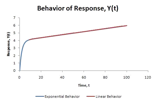
As can be seen clearly from the graph, initially the systemic response shows more exponential characteristics. However, as time progresses, linear behavior dominates.