7.3: Second-order Differential Equations

Introduction

We consider the general Second-order differential equation:

\[\tau^{2} \frac{d^{2} Y(t)}{d t^{2}}+2 \zeta \tau \frac{d Y(t)}{d t} + Y(t)=X(t) \nonumber \]

If you expand the previous Second-order differential equation:

\[ \begin{align*} \tau_{1} \tau_{2} \frac{d^{2} Y(t)}{d t^{2}}+\left(\tau_{1}+\tau_{2}\right) \frac{d Y(t)}{d t} + Y(t) &=X(t) \\[4pt] \left(\tau_{1} \frac{d}{d t}+1\right)\left(\tau_{2} \frac{d}{d t}+1\right) Y(t) &=X(t) \end{align*}  \nonumber \]

where:

\[\tau=\sqrt{\tau_{1} \tau_{2}} \nonumber \]

\[\zeta=\frac{\tau_{1}+\tau_{2}}{2 \sqrt{\tau_{1} \tau_{2}}} \nonumber \]

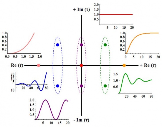
Expansion of the differential equation allows you to guess what the shape of the solution (\(Y(t)\)) will look like when \(X(t)=1\).

The following rules apply when \(τ_1 = Re(τ_1)+ i*Im(τ_1)\) and \(τ_2 = Re(τ_2)+ i*Im(τ_2)\):

• If Re(τ₁) and Re(τ₂) are both positive, and there are NO imaginary parts, \(Y(t)\) will exponentially decay (overdamped).
• If Re(τ₁) and Re(τ₂) are both positive, and there ARE imaginary parts, \(Y(t)\) will oscillate until it reaches steady state (underdamped).
• If Re(τ₁) and Re(τ₂) are both negative, and there are NO imaginary parts, \(Y(t)\) will exponentially grow (unstable).
• If Re(τ₁) and Re(τ₂) are both negative, and there ARE imaginary parts, \(Y(t)\) will oscillate and grow exponentially (unstable).
• If Re(τ₁) and Re(τ₂) are both zero, and there ARE imaginary parts, \(Y(t)\) will oscillate and neither grow nor decay.
• If τ₁ and τ₂ are both zero, \(Y(t)\) is equal to X(t).

Solution of the General Second-Order System (When X(t)= θ(t))

The solution for the output of the system, \(Y(t)\), can be found in the following section, if we assume that the input, \(X(t)\), is a step function \(θ(t)\). The solution will depend on the value of ζ. If ζ is less than one, \(Y(t)\) will be underdamped. This means that the output will overshoot and oscillate. If ζ is equal to one, \(Y(t)\) will be critically damped. This means that the output will reach the steady state value quickly, without overshoot or oscillation. If ζ is greater than one, \(Y(t)\) will be overdamped. This means that the output will not reach the steady state value as quickly as a critically damped system, but there will be no overshoot or oscillation.

Underdamped (ζ<1)

If \(ζ < 1\), the solution is:

\[Y(t)=1-\frac{1}{\sqrt{1-\zeta^{2}}} e^{-\zeta t / \tau} \sin \left(\sqrt{1-\zeta^{2}} \frac{t}{\tau}+\phi\right) \nonumber \]

where:

\[\phi=-\tan ^{-1}\left(\frac{\sqrt{1-\zeta^{2}}}{\zeta}\right) \nonumber \]

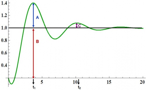
The decay ratio (C/A) can be calculated using the following equation:

\[\frac{C}{A}=e^{-2 \pi \zeta / \sqrt{1-\zeta^{2}}} \nonumber \]

The overshoot (A/B) can be calculated using the following equation:

\[\frac{A}{B}=e^{-\pi \zeta / \sqrt{1-\zeta^{2}}} \nonumber \]

The period (\(T\)) and the frequency (\(ω\)) are the following:

\[T=t_{2}-t_{1}=\frac{2 \pi \tau}{\sqrt{1-\zeta^{2}}} \nonumber \]

\[\omega=\frac{2 \pi}{T}=\frac{\sqrt{1-\zeta^{2}}}{\tau} \nonumber \]

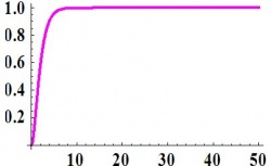
Critically Damped (ζ=1)

If \(ζ = 1\), the solution is:

\[Y(t)=1-\left(1+\frac{t}{\tau}\right) e^{-t / \tau} \nonumber \]

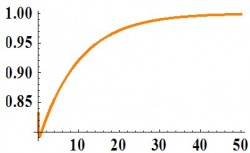
Overdamped (ζ>1)

If \(ζ > 1\), the solution is:

\[Y(t)=1-\frac{1}{\sqrt{\zeta^{2}-1}} e^{-\zeta t / \tau} \sinh \left(\sqrt{\zeta^{2}-1} \frac{t}{\tau}+\phi\right) \nonumber \]

where:

\[\phi=-\tanh ^{-1}\left(\frac{\sqrt{\zeta^{2}-1}}{\zeta}\right) \nonumber \]

Example \(\PageIndex{1}\)

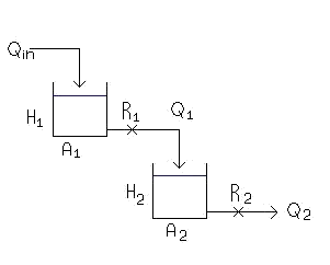
Given:

• A₁ = 1 m²
• A₂ = 1.5 m²
• R₁ = 0.25 s/m²
• R₂ = 0.75 s/m²

where:

• A is the area of the tank
• Q is the volumetric flowrate
• R is the resistance to the flow of the stream exiting the tank
• H is the height of liquid in the tank

develop an expression describing the response of H₂ to Q_in. Determine if the system is over, under or critically damped and determine what the graph of the expression would look like using the complex τ plane above. A diagram of the system is shown below:

Solution

Performing a mass balance on each tank:

\[A_{1} \frac{d H_{1}}{d t}=Q_{i n}-\frac{H_{1}}{R_{1}} \label{1} \]

\[A_{2} \frac{d H_{2}}{d t}=\frac{H_{1}}{R_{1}}-\frac{H_{2}}{R_{2}} \label{2} \]

where the left hand terms account for the accumulation in the tank and the right hand terms account for the flow in the entering and exiting streams

Let τ₁ = R₁A₁ and τ₂ = R₂A₂

Equations \ref{1} and \ref{2} now become

\[\tau_{1} \frac{d H_{1}}{d t}=R_{1} Q_{i n}-H_{1} \label{3} \]

\[\tau_{2} \frac{d H_{2}}{d t}=\frac{R_{2}}{R_{1}} H_{1}-H_{2} \label{4} \]

Put like terms on the same side and factor

\[\left(\tau_{1} \frac{d}{d t}+1\right) H_{1}=R_{1} Q_{i n} \label{5} \]

\[\left(\tau_{2} \frac{d}{d t}+1\right) H_{2}=\frac{R_{2}}{R_{1}} H_{1} \label{6} \]

Apply \(\left(\tau_{1} \frac{d}{d t}+1\right)\) operator from Equation \ref{5} to Equation \ref{6}

\[\left(\tau_{1} \frac{d}{d t}+1\right)\left(\tau_{2} \frac{d}{d t}+1\right) H_{2}=\left(\tau_{1} \frac{d}{d t}+1\right) \frac{R_{2}}{R_{1}} H_{1} \label{7} \]

The \(\left(\tau_{1} \frac{d}{d t}+1\right) H_{1}\) term from the left hand portion of Equation \ref{5} can be substituted into the right hand side of Equation \ref{7}

\[\left(\tau_{1} \frac{d}{d t}+1\right)\left(\tau_{2} \frac{d}{d t}+1\right) H_{2}=R_{1} Q_{i n} \frac{R_{2}}{R_{1}} \nonumber \]

\[\left(\tau_{1} \frac{d}{d t}+1\right)\left(\tau_{2} \frac{d}{d t}+1\right) H_{2}=Q_{i n} R_{2} \nonumber \]

This expression shows the response of H₂ to Q_in as a second order solution like those pictured above. Here Y(t)=H₂ and X(t)=R₂ Q_in

\[\zeta=\frac{\tau_{1}+\tau_{2}}{2 \sqrt{\tau_{1} \tau_{2}}}=\frac{(0.25 * 1)+(0.75 * 1.5)}{2 \sqrt{(0.25 * 1)(0.75 * 1.5)}}=1.296 \nonumber \]

Overdamped.

Both values of \(τ\) are positive real numbers, and the behavior of the graph of the equation can be found on the complex τ plane above.

Example \(\PageIndex{2}\): Analogy to Physics - Spring System

It might be helpful to use a spring system as an analogy for our second order systems.

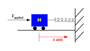
From Newton's second law of motion,

\[F = ma \nonumber \]

where:

• \(F\) is Force
• \(m\) is mass
• \(a\) is acceleration

For the spring system, this equation can be written as:

\[F_{\text {applied}}-F_{\text {friction}}-F_{\text {restoring}}=m x^{\prime \prime} \nonumber \]

where \(x'\) is the acceleration of the car in the x-direction

\[F_{\text {applied}}-f x-k x=m x^{\prime \prime} \nonumber \]

where:

• k is the spring constant, which relates displacement of the object to the force applied
• f is the frequency of oscillation

\[\frac{m}{k} x^{\prime \prime}+\frac{f}{k} x^{\prime}+x=F_{a p p l i e d} \nonumber \]

As you can see, this equation resembles the form of a second order equation. The equation can be then thought of as:

\[\mathrm{T}^{2} X^{\prime \prime}+2 \zeta \mathrm{T} X^{\prime}+X=F_{\text {applied }} \nonumber \]

\[\tau=\sqrt{\frac{m}{k}} \nonumber \]

\[\zeta=\frac{f}{2 \sqrt{m k}} \nonumber \]

Because of this, the spring exhibits behavior like second order differential equations:

• If \(ζ > 1\) or \(f>2 \sqrt{m k}\) it is overdamped
• If \(ζ = 1\) or \(f = 2 \sqrt{m k}\) it is critically damped
• If \(ζ < 1\) or \(f < 2 \sqrt{m k}\) it is underdamped