10.1: Finding fixed points in ODEs and Boolean models

Last updated
Save as PDF

Page ID: 22636

$ \newcommand{\vecs}[1]{\overset { \scriptstyle \rightharpoonup} {\mathbf{#1}} } $ $ \newcommand{\vecd}[1]{\overset{-\!-\!\rightharpoonup}{\vphantom{a}\smash {#1}}} $$\newcommand{\id}{\mathrm{id}}$ $ \newcommand{\Span}{\mathrm{span}}$ $ \newcommand{\kernel}{\mathrm{null}\,}$ $ \newcommand{\range}{\mathrm{range}\,}$ $ \newcommand{\RealPart}{\mathrm{Re}}$ $ \newcommand{\ImaginaryPart}{\mathrm{Im}}$ $ \newcommand{\Argument}{\mathrm{Arg}}$ $ \newcommand{\norm}[1]{\| #1 \|}$ $ \newcommand{\inner}[2]{\langle #1, #2 \rangle}$ $ \newcommand{\Span}{\mathrm{span}}$ $\newcommand{\id}{\mathrm{id}}$ $ \newcommand{\Span}{\mathrm{span}}$ $ \newcommand{\kernel}{\mathrm{null}\,}$ $ \newcommand{\range}{\mathrm{range}\,}$ $ \newcommand{\RealPart}{\mathrm{Re}}$ $ \newcommand{\ImaginaryPart}{\mathrm{Im}}$ $ \newcommand{\Argument}{\mathrm{Arg}}$ $ \newcommand{\norm}[1]{\| #1 \|}$ $ \newcommand{\inner}[2]{\langle #1, #2 \rangle}$ $ \newcommand{\Span}{\mathrm{span}}$$\newcommand{\AA}{\unicode[.8,0]{x212B}}$

Authors: Nicole Blan, Jessica Nunn, Pamela Anne Roxas, Cynthia Sequerah
Stewards: Matthew Kerry Braxton-Andrew, Josh Katzenstein, Soo Kim, Karen Staubach

Introduction

Engineers can gain a better understanding of real world scenarios by using various modeling techniques to explain a system's behavior. Two of these techniques are ODE modeling and Boolean modeling. An important feature of an accurate ODE model is its fixed point solutions. A fixed point indicates where a steady state condition or equilibrum is reached. After locating these fixed points in a system, the stability of each fixed point can be determined (see subsequent Wikis). This stability information enables engineers to ascertain how the system is functioning and its responses to future conditions. It also gives information on how the process should be controlled and helps them to choose the type of control that will work best in achieving this.

Concept Behind Finding Fixed Point

A fixed point is a special system condition where the measured variables or outputs do not change with time. In chemical engineering, we call this a steady state. Fixed points can be either stable or unstable. If disturbances are introduced to a system at steady state, two different results may occur:

the system goes back to those original conditions (stable point)
the system deviates from those conditions rapidly (unstable point)

Subsequent wiki articles will discuss these different types of fixed points in more detail. The focus of this article will be simply finding fixed points, not classifying them. We will discuss several methods of finding fixed points, depending on the type of model employed.

ODE Model

When a process or system is modeled by an ODE or a set of ODEs, the fixed points can be found using various mathematical techniques, from basic hand calcuations to advanced mathematical computer programs. Independent of the method used, the basic principle remains the same: The ODE or set of ODEs are set to zero and the independent variables are solved for. At the points where the differential equations equal zero there is no change occurring. Thus, the solutions found by setting the ODEs equal to zero represent the numerical values of independent variables (i.e. temperature, pressure, concentration) at steady state conditions. If a single ODE or set of ODEs becomes too complicated to be solved by hand, a mathematical program such as Mathematica can be used to find fixed points. The latter part of this article focuses on how to use Mathematica to find fixed points of complicated systems of ODEs.

Note that in some cases there may not be an analytical method to find a fixed point. This case commonly occurs when the solution to a fixed point involves a high degree polynomial or another mathematical function that does not have an analytical inverse. In these cases, we can still find fixed points numerically if we have the parameters.

Boolean Model

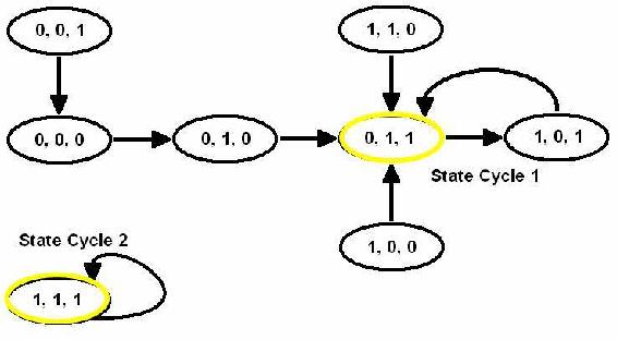
A Boolean Model, as explained in “Boolean Models,” consists of a series of variables with two states: True (1) or False (0). A fixed point in a Boolean model is a condition or set of conditions to which the modeled system converges. This is more clearly seen by drawing state transition diagrams.

State Transition Diagram from Boolean Models

From the state transition diagram above, we can see that there are two fixed points in this system: 0,1,1 and 1,1,1. Starting in any state on the diagram and following the arrows, one of these two states will be reached eventually, indicating that the system tends to achieve either of these sets of operating conditions. If slight disturbances are introduced to the system while it is operating at one of these sets of conditions, it will return to 0,1,1 or 1,1,1. Also noted in the state transition diagram are state cycles. The difference between a state cycle and a fixed point is that a state cycle refers to the entire set of Boolean functions and transition points leading to the steady-state conditions, whereas a fixed point merely refers to the one point in a state cycle where steady-state conditions are reached (such points are indicated by a yellow circle in the diagram).

Finding Fixed Points: Four Possible Cases

There are four possible scenarios when finding the fixed points of an ODE or system of ODEs:

One fixed point
Multiple fixed points
Infinite fixed points
No fixed points

One Fixed Point

The first type of ODE has only one fixed point. An example of such an ODE is found in the Modeling of a Distillation Column. An ODE is used to model the energy balance in the nth stage of the distillation column:

\[\frac{d T_{n}}{d t}=\frac{1}{M_{W}}\left[L_{n-1} x_{n-1}-W x_{W}\right]\left[T_{n-1}-T_{n}\right]+\frac{q_{r}}{M_{W} c_{p}} \nonumber \]

Which can also be written as:

\[\frac{d T_{n}}{d t}-\frac{1}{M_{W}} \left[ L_{n-1} x_{n-1}-W x_{W}\right]\left[T_{n-2}\right]+\frac{q_{r}}{M_{W} c_{p}}+\frac{1}{M_{W}}\left[L_{n-1} x_{n-1}-W x_{W}\right]\left[-T_{n}\right] \nonumber \]

If initial conditions i.e. T_n_{− 1},L_n_{− 1},x_n_{− 1} are known, the equation above reduces to:

\[\frac{d T_{n}}{d t}=a+b T_{n} \nonumber \]

where $a$ and $b$ are constants since all the variables are now known.

\[a=\frac{1}{M_{W}}\left[L_{n-1} x_{n-1}-W x_{W}\right]\left[T_{n-1}\right]+\frac{q_{r}}{M_{W} c_{p}} \nonumber \]

\[b=\frac{-1}{M_{W}}\left[L_{n-1} x_{n-1}-W x_{W}\right] \nonumber \]

By analyzing the equation

\[\frac{d T_{n}}{d t}=0=a+b T_{n} \nonumber \]

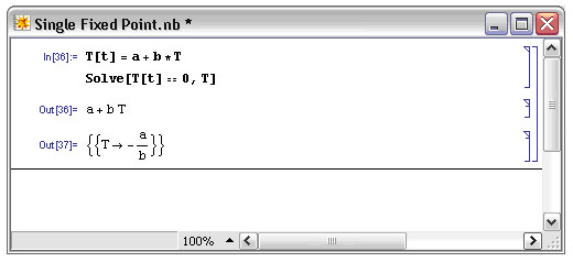
we can immediately deduce that at steady state $T_n = - a/b$. Clearly, there is only one fixed point in this system, only one temperature of the distillation column which will be at steady-state conditions. We can use Mathematica to solve for the fixed point of this system and check our results. In Mathematica, the Solve[] function can be used to solve complicated equations and systems of complicated equations. There are some simple formatting rules that should be followed while using Mathematica:

Type your equation and let the differential be called an arbitrary variable (e.g. T[t])
Type Solve[T[t]==0,T] and hit Shift+Enter
This produces an output contained inside curly brackets

Please read the Solving ODEs with Mathematica section for more information on syntax and functions.

A sample of how the format in Mathematica looks like is shown below:

ingle fixed point.jpg

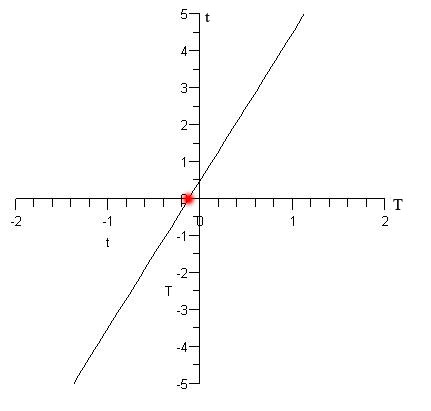
Maple can be used to visualize a single fixed point. Wherever the plot intersects the x-axis represents a fixed point, because the ODE is equal to zero at that point.

The following Maple syntax was used to plot the ODE: plot(0.5+4t, t=-2..2,T=0..5,color=black);

The constant a = 0.5 and the constant b = 4 in the above example.

The resulting graph is below, the red point indicates at what T a fixed point occurs:

ne more.jpg

Solving a single fixed point for an ODE and a controller in Mathematica

Identify what type of controller it is (P, I , PI, or PID etc.)
Identify your ODE equations (Is the controller a function of the ODE?)

Example: Solve for the fixed points given the three differential equations and the two controllers (u1 and u2).

\[\left.\frac{d H}{d t}=(1 / A) (F(i n)-F_{out}\right)\right) \nonumber \]

\[\left.\frac{\left.d F_{in} \right)}{d t}=K(v 1)\left(u_{1}\right) \nonumber \]

\[\left.\frac{\left.d F_{out}\right)}{d t}=K_{(v2} \right)\left(u_{2}\right) H \nonumber \]

Where H is the level in the tank, $F_{in}$ is the flow in, $F_{out}$ the flow out, and $u_1$ and $u_2$ are the signals to the valves $v_1$ and $v_2$. $Kv1$ and $Kv2$ are valve gains (assumed to be linear in this case, although this does not have to be). Note that the exit flow also depends on the depth of fluid in the tank.

You next parameterize your model from experimental data to find values for the constants:

A=2.5 meters squared

K_(v1)=0.046 meters cubed/(minute mA)

K_(v2)=0.017 meters squared/(minute mA)

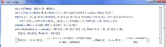
Next you want to add:

A full PID controller to regulate Fout via FC1 connected to v2.
A P-only controller to regulate H via LC1 connected to v1.

For this system you want to maintain the tank level at 3 meters and the exit flow (Fset) at 0.4 m3 /minute. The following Mathematica code should look as follows:

Multiple Fixed Points

Multiple fixed points for an ODE or system of ODEs indicate that several steady states exist for a process, which is a fairly common situation in reactor kinetics and other applications. When multiple fixed points exist, the optimal steady-state conditions are chosen based on the fixed point's stability and the desired operating conditions of the system.

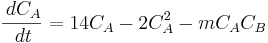
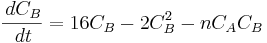
The following is an example of a system of ODEs with multiple fixed points:

\[\frac{d C_{A}}{d t}=14 C_{A}-2 C_{A}^{2}-C_{A} C_{B} \nonumber \]

\[\frac{d C_{B}}{d t}=16 C_{B}-2 C_{B}^{2}-C_{A} C_{B} \nonumber \]

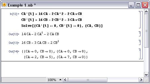
The above system of ODEs can be entered into Mathematica with the following syntax:

ultiple Fixed Points.jpg

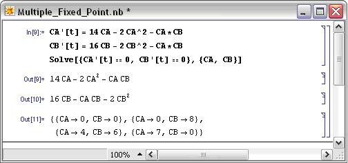
This system in particular has four fixed points. Maple can be used to visualize the fixed points by using the following syntax:

with(plots):

fieldplot([14*x-2*x^2-x*y,16*y-2*y^2-x*y],x=0..10,y=0..10,fieldstrength=log);

The first line initializes the plotting package within Maple that allows for plotting vector fields. The second line uses the command “fieldplot” and inputs the two ODEs that make up the system. The scales of the x and y-axis are set to range from 0 to 10. The fieldstrength command is mainly used for visual purposes, so that the direction of the arrows becomes more apparent. Below is the resulting plot:

ultiple Fixed Points Graph.jpg

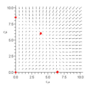
The red dots indicate the fixed points of the system. On the plot, these points are where all the surrounding arrows converge or diverge. Converging arrows indicate a stable fixed point, in this example the point at (4,6) is a stable fixed point. Diverging arrows indicate an unstable fixed point, in this example (0,0), (0,8) and (7,0) are unstable fixed points.

Infinite Fixed Points

An example of an ODE with infinite fixed points is an oscillating ODE such as:

$frac{\,dy}{\,dx}=cos(ax)$

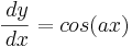
where a is a constant.

Using Mathematica to solve for the fixed points by setting

$frac{\,dy}{\,dx}=0=cos(ax)$

nfinitte fixed points.JPG

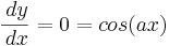
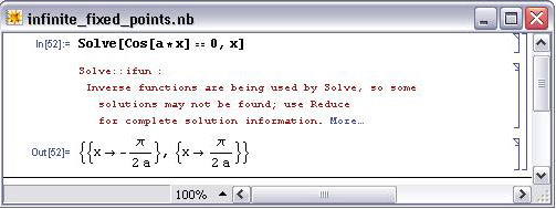
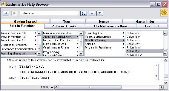
If you click the "More" link on Mathematica it will basically state that there are other solutions possible according to the Help section shown below:

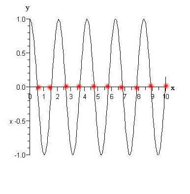
The Maple syntax used to graph the solved differential equation is:

plot(cos(3t),t=0..10,T=-1..1,color=black);

The constant a = 3 in this case.

The infinite fixed points can be seen in the graph below, where anytime the function crosses the x axis, we have a fixed point:

No Fixed Points

The fourth type of ODE does not contain fixed points. This occurs when a certain variable (such as temperature or pressure) has no effect on a system regardless of how it changes. Generally, systems with this sort of behavior should be avoided because they are difficult to control as they are always changing.

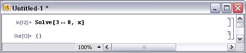
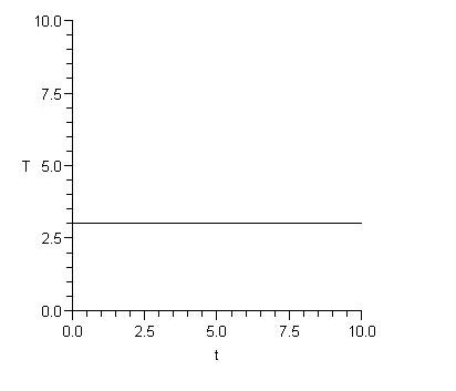
This can be modeled by vertical or horizontal lines due to the fact that no fixed points are found by setting the line equal to zero. An ODE is used to model a line held constant at a:

$frac{\,dT}{\,dt}=a$

Where, a can be any constant except 0.

Intuitively, trying to find a fixed point in this system is not possible, because a constant such as 3 can never equal zero. Solving this ODE is not possible even by analyzing the system. Therefore, when inputting this into Mathematica, it yields {}. The notation {} means that there are no fixed points within the system. The image below is how Mathematica solves the ODE.

o Fixed Points.jpg

By using Maple (version 10), one can visually see a lack of fixed points by using the following syntax:

plot(3, t = 0..10, T = 0..10, color = black);

The constant a = 3 in the above case.

This image shows that the line is horizontal and never crosses the x axis, indicating a lack of fixed points.

Summary

A fixed point is a system condition where the measured variables or outputs do not change with time. These points can be stable or unstable; refer to Using Eigenvalues to evaluate stability for an introduction to a common method for determining stability of fixed points.

There are four possible cases when determining fixed points for a system described by ODEs:

One fixed point
Multiple fixed points
Infitite fixed points
No fixed points

There are methods described above for using Mathematica or Maple to solve for the fixed points in each case. Fixed points can also be determined for a Boolean model.

Knowing the fixed points of a system is very important when designing a control architecture for the system. These are the operating conditions that the system will exhibit at steady-state. Controllers can have influence on the fixed points, so a thorough analysis of fixed points using equations describing the system and the controllers should be conducted before implementation of the control scheme.

Worked out Example 1: Manipulating a System of Equations

Recall the example system of ODEs used in the Multiple Fixed Points Section:

$frac{\,dC_A}{\,dt}= 14C_A-2C_A^2-mC_AC_B$

$frac{\,dC_B}{\,dt}= 16C_B-2C_B^2-nC_AC_B$

Find how the fixed points change when m = 2 and n = 3.

Solution

xample 1 problem solution.jpg

Worked out Example 2: System of ODEs

You are asked to estimate the fixed point(s)of a heat exchanger in your plant. The fixed points corresponds to the temperatures of your tube-side (hot) and shell-side (cold) fluids respectively, T_t_,_out and T_s_,_out. Neglect heat loss to the surrounding area i.e. 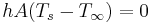$A(T_{s}- T_{\infty})=0$ .

Given the two main ODEs used to model a heat exchanger, use Mathematica to solve for the fixed points of the system in terms of the known variables.

$mc_{p}\frac{dT_{t,out}}{dt}=\rho c_{p}F_{t, in}T_{t, in}-\rho c_{p}F_{t, out}T_{t, out}- \frac {kA}{\Delta z} (T_{t, out} - T_{s,out})$ (equation 1)

$mc_{p}\frac{dT_{s, out}}{dt}=\rho c_{p}F_{s, in}T_{s, in}-\rho c_{p}F_{s, out}T_{s, out}- \frac {kA}{\Delta z} (T_{s, out} - T_{t, out})- hA(T_{s}- T_{\infty})$ (equation 2)

The values for m, c_p, ρ, F_t_,_in, F_t_,_out, k, A, δz, and T_t_,_in, F_s_,_in, F_s_,_out, T_s_,_in are given and fixed.

Please refer to the Wiki article on HeatExchangeModel for detailed explanation on the meaning of the variables and the derivation of the ODEs above.

Hint: Lump up all known variables under one general variable

Solution

Simplify the 2 equations to the ODEs below:

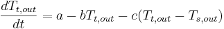$frac{dT_{t,out}}{dt}=a-bT_{t, out}-c(T_{t, out} - T_{s,out})$ (equation 1a)

$frac{dT_{s,out}}{dt}=d-eT_{s, out}-f(T_{s, out} - T_{t,out})$ (equation 2a)

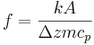
where 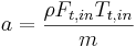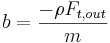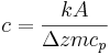$=\frac {\rho F_{t, in}T_{t, in}}{m}$ , $=\frac {-\rho F_{t, out}}{m}$ , $=\frac {kA}{\Delta zmc_p}$ and $=\frac {\rho F_{s, in}T_{s, in}}{m}$ , $=\frac{\rho F_{s, out}}{m}$ , $=\frac {kA}{\Delta zmc_p}$

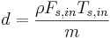Type these equation into Mathematica using the appropriate syntax and use the Solve[] function to find the fixed points.

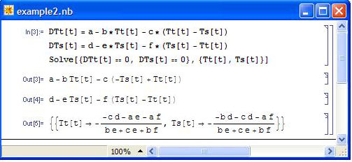
We have found our fixed point. Just plug in the variables as defined earlier for a, b, c, d, e, f and you will obtain the temperatures in terms of the useful parameters.

Multiple Choice Question 1

The solutions found by setting the ODE equal to zero represent:

a) independent variables not at steady state conditions

b) dependent variables not at steady state conditions

c) independent variables at steady state conditions

d) dependent variables at steady state conditions

Answer: C

Multiple Choice Question 2

How many fixed points are there when the following equation is solved by Mathematica?

$frac{\,dT}{\,dt}= 8t-4t^2-t^3$

a) none

b) 1

c) 2

d) 3

Answer: D

Sage's Corner

Stability of Fixed Points
video.google.com/googleplayer...80917022362654

slides for this talk

References

Edwards H., Penney D.(2003), Differential Equations: Computing and Modeling, Third Edition. Prentice-Hall. ISBN 0130673374
Strogatz, Steven H.(2001), Nonlinear Dynamic and Chaos: With Applications to Physics, Biology, Chemistry, and Engineering, 1st Edition. Addison-Wesley. ISBN 0738204536