
10.5: Phase Plane Analysis - Attractors, Spirals, and Limit cycles
- Page ID
- 22504

Introduction to Attractors, Spirals and Limit Cycles
We often use differential equations to model a dynamic system such as a valve opening or tank filling. Without a driving force, dynamic systems would stop moving. At the same time dissipative forces such as internal friction and thermodynamic losses are taking away from the driving force. Together the opposing forces cancel any interruptions or initial conditions and cause the system to settle into typical behavior. Attractors are the location that the dynamic system is drawn to in its typical behavior. Attractors can be fixed points, limit cycles, spirals or other geometrical sets.
Limit cycles are much like sources or sinks, except they are closed trajectories rather than points. Once a trajectory is caught in a limit cycle, it will continue to follow that cycle. By definition, at least one trajectory spirals into the limit cycle as time approaches either positive or negative infinity. Like a sink, attractive (stable) limit cycles have the neighboring trajectories approaching the limit cycle as time approaches positive infinity. Like a source, non-attractive (unstable) limit cycles have the neighboring trajectories approaching the limit cycle as time approaches negative infinity. Below is an illustration of a limit cycle [1].

Spirals are a similar concept. The attractor is a spiral if it has complex eigenvalues. If the real portion of the complex eigenvalue is positive (i.e. 3 + 2i), the attractor is unstable and the system will move away from steady-state operation given a disturbance. If the real portion of the eigenvalue is negative (i.e. -2 + 5i), the attractor is stable and will return to steady-state operation given a disturbance.
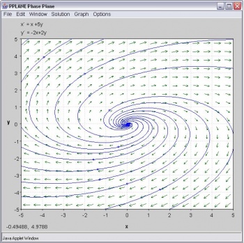
Given the following set of linear equations we will walk through an example that produces a spiral:
\[\begin{align*}
\frac{d x}{d t}&=2 x+5 y \\
\frac{d y}{d t}&=-5 x+2 y
\end{align*} \nonumber \]
The Jacobian matrix would be the coefficients:
\[A=\left|\begin{array}{cc}
2 & 5 \\
-5 & 2
\end{array}\right| \nonumber \]
Next we found the eigenvalues:
\[(A-\lambda I)=\left|\begin{array}{cc}
2 & 5 \\
-5 & 2
\end{array}\right|-\lambda\left|\begin{array}{cc}
1 & 0 \\
0 & 1
\end{array}\right|=\left|\begin{array}{cc}
(2-\lambda) & 5 \\
-5 & (2-\lambda)
\end{array}\right| \nonumber \]
where \(I\) is the identity matrix
\[I = \left|\begin{array}{ll}
1 & 0 \\
0 & 1
\end{array}\right| \nonumber \]
\[\operatorname{det}(A-\lambda I)=(2-\lambda)^{2}+25=0 \nonumber \]
Eigenvalues:
\[\lambda=2 \pm 5 i \nonumber \]
The system is unstable because the real portion of the complex eigenvalues is positive.
To find the first eigenvector we continue by plugging in \(2 − 5i\):
\[\left|\begin{array}{cc}
(2-\lambda) & 5 \\
-5 & (2-\lambda)
\end{array}\right|=\left|\begin{array}{cc}
2-(2-5 i) & 5 \\
-5 & 2-(2-5 i)
\end{array}\right|=\left|\begin{array}{cc}
5 i & 5 \\
-5 & 5 i
\end{array}\right| \nonumber \]
\[(A-\lambda I) v=\left|\begin{array}{cc}
5 i & 5 \\
-5 & 5 i
\end{array}\right| v=0 \nonumber \]
let
\[v=\left|\begin{array}{l} x \\ y \end{array}\right| \nonumber \]
\[\left|\begin{array}{cc}
5 i & 5 \\
-5 & 5 i
\end{array}\right|\left|\begin{array}{l}
x \\
y
\end{array}| = |\begin{array}{l}
0 \\
0
\end{array}\right| \nonumber \]
We now have a system of equations which we can solve for x, y:
\begin{align*}
5 i x+5 y & =0 \\
-5 x+5 i y & =0
\end{align*}
Dividing both equations by 5:
\[\begin{align*}
i x+y & =0 \\
-x+i y & =0
\end{align*} \nonumber \]
Solution
\[v_{1}=\left|\begin{array}{c}
-1 \\
i
\end{array}\right| \nonumber \]
Following the same procedure using the second eigenvalue of 2 + 5i, we find the second eigenvector to be:
\[v_{2}=\left|\begin{array}{c}
i \\ -1
\end{array}\right| \nonumber \]
Now plugging both eigenvalues and eigenvectors into the characteristic equation:
\[\begin{align*}
x(t)&=e^{2 t}\left(C_{1} \cos 5 t+C_{2} \sin 5 t\right) \\
y(t)&=e^{2 t}\left(C_{3} \cos 5 t+C_{4} \sin 5 t\right)
\end{align*} \nonumber \]
For more on this procedure, see: Eigenvalues and Eigenvectors
The phase-plane plot is shown below:
Introduction to Pplane
Phase-plane analysis is an important tool in studying the behavior of nonlinear systems since there is often no analytical solution for a nonlinear system model.
PPlane is a JAVA applet for phase plane analysis of two-dimensional systems. It starts in your web browser and you can directly input your equations and parameter values. PPLANE plots vector fields for systems of differential equations. At each point, (x,y), of a grid, PPLANE draws an arrow indicating the direction and magnitude of the vector (x',y'). This vector equals dy/dt / dx/dt = dy/dx, and is independent of t; therefore, it must be tangent to any solution curve through (x,y).
It allows the user to plot solution curves in the phase plane by simple clicking on them. It also enables the user to plot these solutions in a variety of plots. There are a number of advanced features, including finding equilibrium points, eigenvalues and nullclines, that you will find useful later.
How to use Pplane
In the PPlane equation window you can enter a system of differential equations of the form \(dx/dt = f(x,y)\) and \(dy/dt = g(x,y)\), define parameters and resize the display window. Under the Gallery pull down from the menu, you can switch to a linear system.
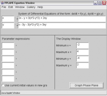
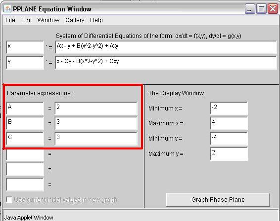
Note, if your differential equations contain constant parameters, you can enter them in the "Parameter Expressions" boxes below the differential equations as seen in the figure below (A, B, and C are used as example parameters). This is a convenient feature to use when considering the effect of changed parameters on the steady state of a system because it eliminates the redundancy of re-entering the parameter values multiple times within the differential equations.
In the PPlane Phase Plane window below you will see the vector fields for the system. By clicking on the field you will plot solution curves in the phase plane. If you are interested in a plot of your solution vs. time or a 3-D view, click on graph:
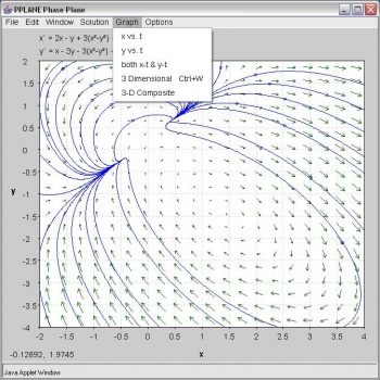
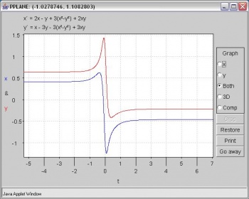
If you choose the x-t and y-t option, you have to pick a specific solution curve. The result will look like this:
Use the crop function to zoom in on a point of interest
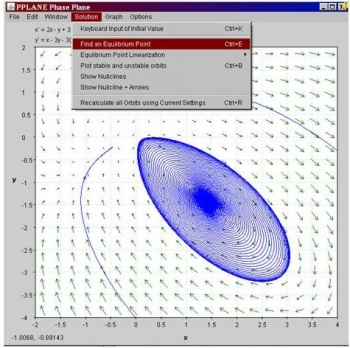
Choose Find Equillibrium Point under the Solution pull down menu. Then when you click on an orbit in the phaseplane, the Pplane Messages window will display the eigenvalues and possible equillibrium points.
Additional Things you can Change in PPlane
Changing the Slope Field
By clicking on the "Options" tab, then by selecting "Direction Field Settings," you can change the number of rows and columns plotted, the way the field is made up, as well as the computational settings of PPlane.
Erasing Made Orbits
On the "Edit" tab, there are options that say "Delete Orbit" or "Delete All Orbits". These options act as their names imply.
Changing the Direction of Graphing
By clicking on the "Options" tab, then by selecting the "Solution Direction" option, you can then change the way that PPlane graphs a line when you click on the field. You can change the graphing to plot forwards (for values of t>0), backwards (for values of t<0) or in both directions of t.
More Uses for PPLANE
Of the many uses that PPLANE has to offer, some of the most helpful functions involve:
Finding eigenvalues/eigenvectors for an equilibrium point.
After graphing a series of differential equations, find a particular equilibrium point within the graphed data (“Find an Equilibrium Point,” under the Solution tab)
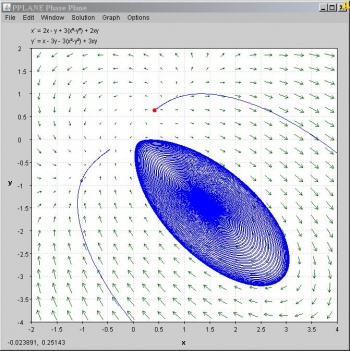
Now, by selecting a point on the field that has ben graphed by pplane, pplane will find the closest equilibrium point on the graph, and highlight this point on the graph in red.
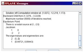
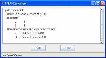
The PPLANE Messages box in the upper left hand corner of the screen should pop up with some new information. This information provides eigenvalues and the corresponding eigenvectors to the selected equilibrium value:
Stability of a Equilibrium Point
Similarly to before, the Messages Box will provide the stability features (ie: is it a nodal sink?) of the found equilibrium point, immediately after using the “Find an Equilibrium Point.”
Other concepts of phase plane analysis
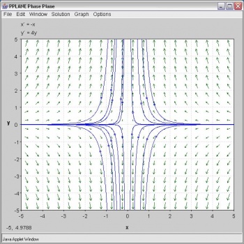
Separatrix
A separatrix is any line in the phase-plane that is not crossed by any trajectory. The unstable equilibrium point, or saddle point, below illustrates the idea of a separatrix, as neither the x or y axis is crossed by a trajectory. If you picture a topographic map, the seperatrix would be a mountain ridge; if you fall a little of the edge, you will never come back. Plotting your phase plane in Pplane would be useful to identify impossible set points, for example.
Nullclines
A nullcline is a curve where x'=0 or y'=0, thus indicating where the phase plane is completely horizontal or completely vertical. The point at which two nullclines intersect is an equilibrium point. Nullclines can also be quite useful for visualization of a phase plane diagram as they split the phase plane into regions of similar flow. To display nullclines on the Phase Plane window, select Nullclines under the Solutions drop down menu. The screenshot below is an example.
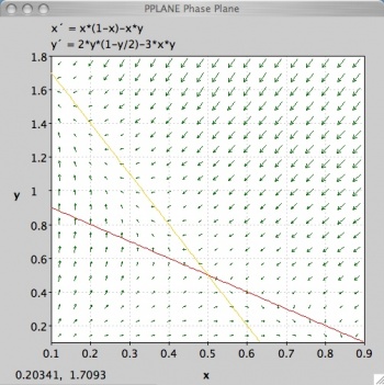
Notice that the red nullcline shows where the flow is completely vertical (x'=0) and the yellow nullcline shows where the flow is completely horizontal (y'=0).
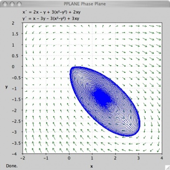
Limit Cycle
Below you will find a solution curve for a limit cycle. The limit cycle contains the response in a set range, which is something you may want to take advantage for certain engineering applications. On the other hand it is always rotating and may not be stable enough for your purposes.
Taking Screen Shots to copy Pplane phase portraits
With the introduction of Windows Vista, the Snipping Tool was introduced. This tool allows much greater flexibility with taking screen shots and editing them. This article will talk about the Snipping Tool as well as the Windows Print Screen key which can be used to take photos of your computer screen. When pressing the key, your computer copies the image of your screen and onto your computer’s clipboard. The image can then be pasted into multiple programs. There are many instances throughout the CHE 466 course in which taking a screen shot of your work will come in handy. Examples include copying phase portraits created in Pplane, graphs created in Mathematica, or your Mathematica code.
To enable the Snipping Tool on your Vista computer go to the Windows button in the bottom left of your screen and click Accessories -> Snipping Tool.
Figure 1. How to enable the Snipping Tool

A window will appear asking if you would like to add the Snipping Tool to your Quicklaunch. This provides a simple and quick way to take screenshots.
To take a picture of your graph, just press the Snipping Tool button in the Quicklaunch area and a window like this will appear:
Figure 2. The Snipping Tool Window
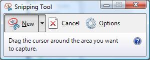
Automatically, the Snipping Tool will default to a crosshair from which you can click and drag to make a selection of the section of the screen you would like represented by a red rectangle.
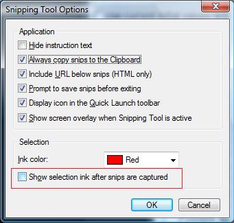
WARNING: In the Options section you should uncheck "Show selection ink after snips are captured" in order to eliminate the red edge around your photos.
Figure 3. Snipping Tool Option Menu (Uncheck the selection ink)
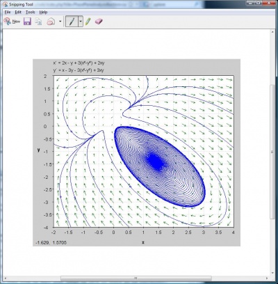
The Snipping Tool will open up a new window with your selection and copy the image to your clipboard. Feel free to edit your image or save it where it is convenient.
Figure 4. Snipping Tool Editing Window
If not using Windows Vista you can still use Print Screen:
Follow these simple steps to copy and paste your phase portrait into a Microsoft Word document:
- Pull up the window containing your phase portrait so that it is displayed on the screen.
- Find the Print Screen or PrtSc button in the upper-right hand portion of your keyboard. (The key may appear slightly different depending on your Windows keyboard manufacturer).
- Open Microsoft Word to the document of your choice (i.e. CHE 466 Homework 7).
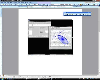
- Paste the image into the Word document. Figure 1 below indicates how your phase portrait will look in Word.
- To crop or resize the image as you like, you may use the Picture toolbar (seen in Figure 2) by selecting View -> Toolbars -> Picture.
If you prefer to take a screen shot of just your phase portrait rather than the entire computer screen, follow these simple steps:
- Pull up the window containing your phase portrait so that it is displayed on the screen.
- Press Alt-Print Screen to capture a photo of the window you selected.
- Open Microsoft Word to the document of your choice (i.e. CHE 466 Homework 7).
- Paste the image into the Word document. Figure 3 below indicates how your phase portrait image will look.
Figure 5. Initial screen shot
Use PPLANE to calculate the following information of the system given below: location and type of equilbrium point, Jacobian matrix, eigenvectors, and eigenvalues.
\[\begin{array}{c}
x^{\prime}=y \\
y^{\prime}=2 x+y
\end{array} \nonumber \]
Solution
Using PPLANE's "Find an Equlibrium Point" feature and clicking on the phase plane, the following equilibrium point will be indicated:
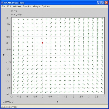
The location, and type of the equilibrium point is given in the "PPLANE Messages" window, along with the Jacobian matrix, eignvectors and eigenvalues.
For our second example problem we would like you to try a non-linear system of equations.
Solve for the set of equations on PPlane. Consider the trends of change in rate of the differential equations and subsequently solve the equations on Mathematica to compare the trends. The following two differential equations are going to be used to walk through the solutions on PPlane and Mathematica:
\[\(\frac{d x}{d t}=x-(5 x y) \nonumber \]
\[\frac{d y}{d t}=-2 x+2 y\) \nonumber \]
Solution
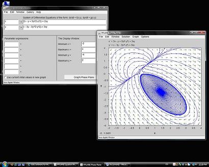
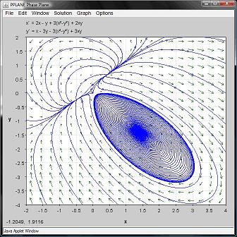
The above equations were put in to the PPlane window and solved. The following two windows show the solution for the set of differential equations:


Looking at the phase-plane plot, at low values of x and y, t increases slowly. However at higher values of y, the increase in t is rapid. When x is high and y is low, however, t increases slowly. Mathematica will help us visualize the relative rates of change better.
The following is the code used in Mathematica to solve and plot the set of differential equations:
ODEs = {x'[t] == (x[t] - 5*x[t]*y[t]), y'[t] == (-2*x[t]) + (2*y[t]), x[0] == 9, y[0] == 370} numericalSol = NDSolve[ODEs, {x[t], y[t]}, {t, 1, 100}] Plot[y[t] /. numericalSol, {t, 1, 100}, PlotRange -> All]
The graphs obtained on Mathematica for x versus t and y versus t are shown below. Please note the difference between the axes scales.

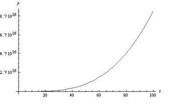
Also, for a closer look, here are the plots of the slopes of graphs above.
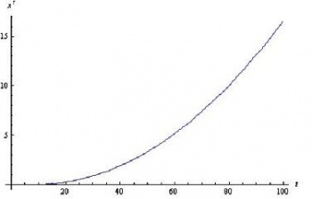
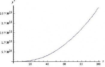
Comparing the increase in t with increase in x, we see a similar trend in the PPlane diagram. Mathematica shows a constantly increasing x' with t. At higher values of x, the value for t increases in the PPlane diagram. However, as seen clearly in the PPlane diagram and the graphs of the slope of x with respect to t and the slope of y with respect to t, the slope of x does not compare to the very large slope shown for y' versus t. Therefore the results using Mathematica and PPlane are consistant.
This modeling system could be used to view trends of variables in a CSTR or any other system which can be modeled using differential equations.
Multiple Choice Questions
Question 1
Open PPLANE and enter the following equations into the PPLANE Equation Window:
x '= sin(x)
y' = cos(y)
What does the resulting phase plane look like? (Note: Click on image to enlarge)
A. 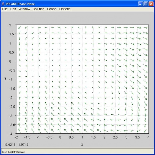
B. 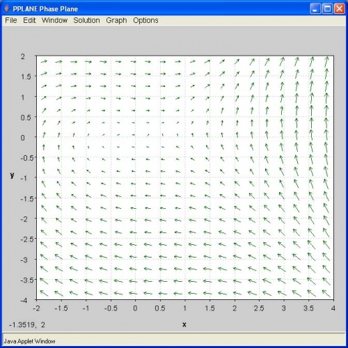
C. 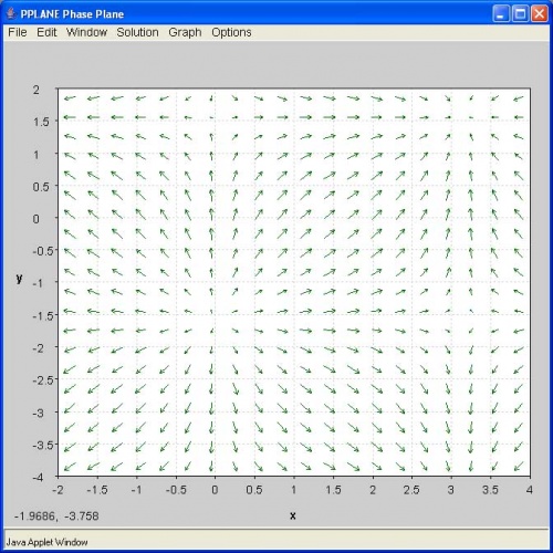
D. 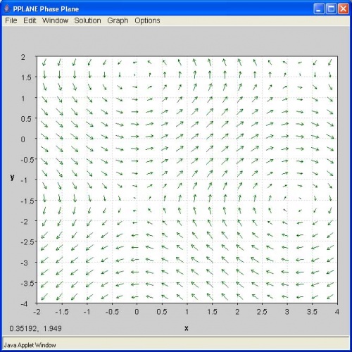
Question 2
If you have a disturbance in your system and the system is driven right back to equilibrium, that fixed point's eigenvalue is most likely a:
A. complex number with negative real number component
B. 0
C. negative real number
D. positive real number
Answers to the Multiple Choice Questions
Question 1: C
Question 2: A
Contributors and Attributions
- Authors: Erin Knight, Dipti Sawalka, Matt Russell, Spencer Yendell
- Stewards: Eric Black, Megan Boekeloo, Daniel Carter, Stacy Young