
13.4: Bayes Rule, Conditional Probability and Independence
- Page ID
- 22525

Introduction
Probability is the likely percentage of times an event is expected to occur if the experiment is repeated for a large number of trials. The probability of rare event is close to zero percent and that of common event is close to 100%. Contrary to popular belief, it is not intended to accurately describe a single event, although people may often use it as such. For example, we all know that the probability of seeing the head side of a coin, if you were to randomly flip it, is 50%. However, many people misinterpret this as 1 in 2 times, 2 in 4 times, 5 in 10 times, etc. of seeing the head side of the coin appear. So if you were to flip a coin 4 times and it came up heads every single time, is this 50% probability incorrect? No! It's just that your sample size is small. If you were to flip a coin 10,000 times, you would begin to see a more even distribution of heads and tails. (And if you don't, you should probably get a different coin.) Now, as engineers, even if we know the probability of the system, we don't have time to perform 10,000 trials to verify it. However, you'd be surprised at the small number of trials that are required to get an accurate representation of the system. The following sections describe the relationship between events and their probabilities. These relationships will then be used to describe another probability theory known as Bayes’ Theorem.
Types of Probability
Combination
Combinatorics is the study of all the possible orderings of a finite number of objects into distinct groups. If we use combinatorics to study the possible combinations made from ordering the letters A, B, and C we can begin by counting out all the orderings
\[\{(A B C),(A C B), (B C A),(B A C), (C B A),(C A B)\} \nonumber \nonumber \]
giving us a total of 6 possible combinations of 3 distinct objects. As you can imagine the counting method is simple when the number of objects is small yet, when the number of objects being analyzed increases the method of counting by hand becomes increasingly tedious. The way to do this mathematically is using factorials. If you have n distinct objects then you can order them into \(n!\) groups. Breaking the factorial down for our first example we can say, first there are 3 objects to choose from, then 2, then 1 no matter which object we choose first. Multiplying the numbers together we get 3*2*1=3!. Now consider finding all the possible orderings using all the letters of the alphabet. Knowing there are 26 letters in the English alphabet, the number of possible outcomes is simply 26!, a number so large that counting would be difficult.
Now what if there are n objects and m that are equivalent and you wish to know the number of possible outcomes. By example imagine finding the number of distinct combinations from rearranging the letters of PEPPER. There are 6 letters, 2 Es and 3 Ps but only 1 R. Starting with 6! we need to divide by the repeat possible outcomes
\[\dfrac{6 !}{3 ! \times 2 !}=\dfrac{6 \times 5 \times 4 \times 3 !}{3 ! \times 2 !}=\dfrac{6 \times 5 \times 4}{2}= 6 \times 5 \times 2=60 \, \text{possible arrangements} \nonumber \nonumber \]
where on the bottom, the \(3!\) is for the repeated Ps and the \(2!\) is for the repeated Es.
You can cancel same integer factorials just like integers.
The next topic of importance is choosing objects from a finite set. For example, if four hockey teams are made from 60 different players, how many teams are possible? This is found using the following relation:
\[ \dfrac{60 \times 59 \times 58 \times 57}{4 \times 3 \times 2 \times 1}=487,635 \, \text{possible teams} \nonumber \nonumber \]
Generally, this type of problem can be solved using this relation:
\[(n, r)=\dfrac{n !}{(n-r) ! r !} \label{choose} \]
called n choose r where \(n\) is the number of objects and \(r\) is the number of groups
Using Equation \ref{choose}, for the example above the math would be:
\[ \begin{align*} \dfrac{60 !}{56 ! \times 4 !} &= \\[4pt] \dfrac{60 \times 59 \times 58 \times 57 \times 56 !}{56 ! \times 4 !} &= \\[4pt] \dfrac{60 \times 59 \times 58 \times 57}{4 !} &= 487,635 \, \text{possible teams} \end{align*}\nonumber \]
Joint Probability
Joint probability is the statistical measure where the likelihood of two events occurring together and at the same point in time are calculated. Because joint probability is the probability of two events occurring at the same time, it can only be applied to situations where more than one observation can be made at the same time. When looking at only two random variables, \(A\) and \(B\), this is called bivariate distribution, however this can be applied to numerous events or random variables being measured at one time (multivariate distribution). The probability of two events, \(A\) and \(B\), both occurring is expressed as:
\[P(A, B)\nonumber \]
Joint probability can also be expressed as:
\[P(A \cap B)\nonumber \]
This is read as the probability of the intersection of \(A\) and \(B\).
If \(A\), \(B\), and \(C\) are independent random variables, then
\[P(A, B, C)=P(A) P(B) P(C)\nonumber \]
Two cards are selected randomly from a standard deck of cards (no jokers). Between each draw the card chosen is replaced back in the deck. What is the probability of choosing a four then a five? Let \(P(A)\) denote the probability that the first card is a four and \(P(B)\) denote the probability that the second card is a five.
Solution
If there are 52 cards in a standard card deck with 4 suits, then \(P(A)=4 / 52 \) and \(P(B)=4 / 52\). Knowing that the events are independent, each probability is multiplied together to find the overall probability for the set of events. Therefore:
\[\begin{align*} P(A, B) &=P(A) \times P(B) \\[4pt] &= \left(\dfrac{4}{52}\right) \left(\dfrac{4}{52} \right) \\[4pt] &=1 / 169 \end{align*}\nonumber \]
The probability of choosing a four then a five from the deck with replacement is 1 out of 169.
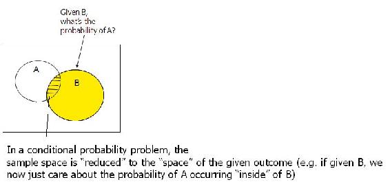
Conditional Probability
Conditional probability is the probability of one event occurring, given that another event occurs. The following expression describes the conditional probability of event \(A\) given that event \(B\) has occurred:
\[P(A \mid B)\nonumber \]
If the events A and B are dependent events, then the following expression can be used to describe the conditional probability of the events:
\[P(A \mid B)=\frac{P(A, B)}{P(B)}\nonumber \]
\[P(B \mid A)=\frac{P(A, B)}{P(A)}\nonumber \]
This can be rearranged to give their joint probability relationship:
\[\begin{align*} P(A, B) &=P(B \mid A) \times P(A) \\[4pt] &=P(A \mid B) \times P(B) \end{align*}\nonumber \]
This states that the probability of events \(A\) and \(B\) occurring is equal to the probability of \(B\) occurring given that \(A\) has occurred multiplied by the probability that \(A\) has occurred.
A graphical representation of conditional probability is shown below:
Conditional probability is often derived from tree diagrams or contingency tables. Suppose you manufacture 100 piston shafts. Event A: feature A is not defective Event B: feature B is not defective
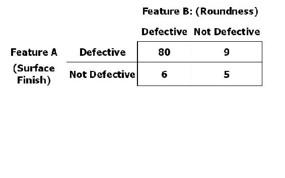
\[P(\text{A Not Def} | \text{B is Def}) = 6 / (80+6) = 0.0698\nonumber \]
\[P(\text{A Not Def} | \text{B Not Def}) = 5 / (9+5) = 0.3571\nonumber \]
Two fair, or unbiased, dice are tossed. Some example outcomes are (1,6) and (3,2). The probability of each possible outcome of the dice is 1/36. When the first die is rolled it results in a value of 2. Once the second die is rolled, what it the probability that the sum of the dice is 7?
Solution
Since it is known that the first value is 2, the possible combination of the two die are as follows:
(2,1) (2,2) (2,3) (2,4) (2,5) (2,6)
This results in six outcomes with equal probabilities since the second die is fair. Therefore, the conditional probability of the outcomes above is 1/6. The conditional probability of the remaining 30 combinations is 0 since the first die is not a 2 in these cases. Finally, since only one of these six outcomes can sum up to 7, (2,5), the probability is 1/6 for rolling a sum of 7 given the value of the first die is a 2.
The probability that a rare species of hamster will give birth to one male and one female is 1/3. The probability that the hamster will give birth to a male is 1/2. What is the probability that the hamster will give birth to a female knowing that the hamster has given birth to a male? Let A denote the probability of giving birth to a male and B denote the probability of giving birth to a female.
Solution
- \(P(A\) is the probability of giving birth to a male
- \(P(B \mid A\) is the probability of giving birth to a female given that birth of a male has already occurred
- \(P(A, A\) is the probability of giving birth to one male and one female
These events are dependent so the following equation must be used:
\[P(A, B)=P(B \mid A) * P(A)\nonumber \]
Rearranging this equation to find \(P(B \mid A\) would give:
\[P(B \mid A)=\frac{P(A, B)}{P(A)}\nonumber \]
Plugging in the known values would give:
\[P(B \mid A)=(1 / 3) /(1 / 2)\nonumber \]
\[P(B \mid A)=2 / 3\nonumber \]
Therefore, the probability of giving birth to a female, given that birth of a male already occurred is 2/3.
Law of Iterative Expectation
An important application of conditional probability is called the "Law of Iterative Expectation".Given simply, it is: E[X]=E[E[X|Y]]. If the random variable distribution of X is unknown, but we are given the distribution of the conditional variable of X, then by finding the expection of the conditional variable twice, we can return to the expectation of the original random variable X. By looking at the expectation of the random variable X, we can deduce the distribution of the random variable X.
The Law of Iterative Expectation is quite useful in mathematics and often used to prove important relationships. Note the example below:
Use the Law of Iterative Expection to find Var[X] given only X|Y.
Solution
E[Var(X|Y)] = E[X^2]-E[(E[X|Y])^2]
Var(E[X|Y)])=E[(E[X|Y])^2]-(E[X])^2
E[Var(X|Y)]+ Var(E[X|Y]) = E[X^2]-E[(E[X|Y])^2] + E[(E[X|Y])^2]-(E[X])^2
Var[X]= E[(E[X|Y])^2] + E[(E[X|Y])^2] (by definition)
thus Var[X] = E[Var(X|Y)]+ Var(E[X|Y])
Marginal Probability
Marginal probability is the unconditional probability of one event; in other words, the probability of an event, regardless of whether another event occurs or not. Finding the marginal probability of an event involves summing all possible configurations of the other event to obtain a weighted average probability. The marginal probability of an event A is expressed as:
\[P(A)=\sum_{B} P(A, B)=\sum_{B} P(A \mid B) * P(B)\nonumber \]
The marginal probability (of A) is obtained by summing all the joint probabilities. Marginal probability can be used whether the events are dependent or independent. If the events are independent then the marginal probability is simplified to simply the probability. The following example will clarify this computation.
The joint probabilities for rain and wind are given in the following table
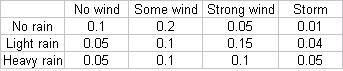
Marginal probability of no rain = sum of Joint probabilities = .1 + .2 + .05+.01 = .36
Similarly, marginal probability of light rain = .05+.1+.15+.04 = .34
Similarly, marginal probability of heavy rain = .3.
Marginalizing Out a Factor
In a system with two or more factors affecting the probability of the output of another factor, one of these initial factors can be marginalized out to simplify calculations if that factor is unknown.
For instance, consider a system where A and B both affect the output of C. If the condition of B is unknown but its probability is known, it can be marginalized out to put the system in terms of how only A affects C, using the equation below:
\[P(C \mid A)=\sum_{i} P\left(C \mid A, B_{i}\right) P\left(B_{i}\right)\nonumber \]
Example Problem 2
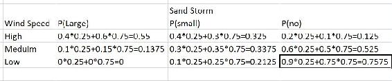
The table below shows the probablitiy of having a large, small or no sand storm, if there is high, medium or no wind, and depending on if there is rain. The next table show the probability of rain.
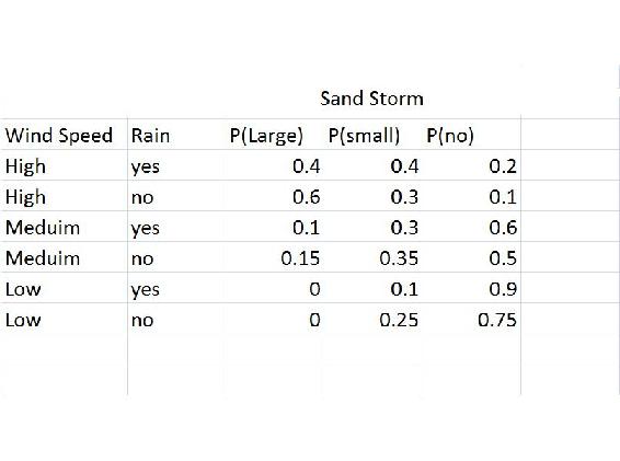
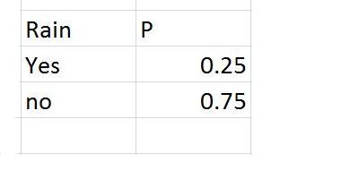
From this it is possible to calculate the probability of a large, small or no sand storm defendant just on the wind speed:
Similarly as to above:
P(Sandstorm Size|Wind Speed)= P(Sandstorm Size|Wind Speed, Rain)*P(Rain)+P(Sandstorm Size|Wind Speed, No Rain)*P(No Rain)
Relationships Between Events
Knowing whether two events are independent or dependent can help to determine which type of probability (joint, conditional, or marginal) can be calculated. In some cases, the probability of an event must be calculated without knowing whether or not related events have occurred. In these cases, marginal probability must be used to evaluate the probability of an event.
Independence
If the two events are considered independent, each can occur individually and the outcome of one event does not affect the outcome of the other event in any way.
Let's say that A and B are independent events. We'll examine what this means for each type of probability.
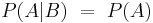
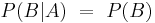
Independence in Conditional Probability
Independent events technically do not have a conditional probability, because in this case, A is not dependent on B and vice versa. Therefore, the probability of A given that B has already occurred is equal to the probability of A (and the probability of B given A is equal to the probability of B). This can be expressed as:
Independence in Joint Probability
Independent events can have a joint probability, even though one event does not rely on the other. For example, joint probability is used to describe an event such as tossing a coin. The outcome when the coin is tossed the first time is not related to the outcome when the same coin tossed a second time. To calculate the joint probability of a set of events we take the product of the individual probabilities of each event in the set. This can be expressed as:
Independent events can also occur in a case where there are three events. For example, if two dice are being rolled with a sum of 6 (Event A). Let event B represent that the first die is a 1 and let event C represent that the second rolled die is a 5. To prove if these events are independent, the following relation is considered:

If any of these relations are false than the event is not independent. When considering events of more than three, the same relation would follow but with an additional relation to event D.
Dependence
If the two events are considered dependent, then the outcome of the second event depends on the probability of the first event. The probabilities of the individual events must be analyzed with conditional probability.
Let's now say that A and B are dependent events. We'll examine what this means for each type of probability.
Dependence in Conditional Probability
Conditional probability only applies to dependent events. In other words, A must depend on B in order to determine the probability of A occurring given that B has already occurred. Therefore, for dependent events A and B, one can just apply the equations as seen in the conditional probability section.
\[P(A \mid B)=\frac{P(A, B)}{P(B)}\nonumber \]
and
\[P(B \mid A)=\frac{P(A, B)}{P(A)}\nonumber \]
Dependence in Joint Probability
Joint probability can also be calculated for dependent events. For example, dependent joint probability can be used to describe cards being drawn from a deck without replacing the cards after each consecutive drawing. In this case, the probability of \(A\) and \(B\) happening is more complex, since the probability of the \(B\) happening depends on the probability of \(A\) happening. It can be expressed as:
\[P(A, B)=P(A) P(B \mid A)\nonumber \]
Note that this equation is found by rearranging the conditional probability equation.
Bayes’ Theorem
Most probability problems are not presented with the probability of an event "A," it is most often helpful to condition on an event A"." At other times, if we are given a desired outcome of an event, and we have several paths to reach that desired outcome, Baye’s Theorem will demonstrate the different probabilities of the pathes reaching the desired outcome. Knowing each probability to reach the desired outcome allows us to pick the best path to follow. Thus, Baye’s Theorem is most useful in a scenario of which when given a desired outcome, we can condition on the outcome to give us the separate probabilities of each condition that lead to the desired outcome.
The following is Bayes' Theorem:
\[P\left(B_{j} \mid A\right)=\frac{P\left(A \mid B_{j}\right) P\left(B_{j}\right)}{\sum_{j} P\left(A \mid B_{j}\right) P\left(B_{j}\right)} \label{Bayes} \]
where \(P\left(A \mid B_{j}\right)\) is the probability of \(A\) conditioned on \(B_j\) and \(\sum_{j} P\left(A \mid B_{j}\right) P\left(B_{j}\right)\) is the law of total probability.
Derivation of Bayes’ Theorem
The derivation of Bayes’ theorem is done using the third law of probability theory and the law of total probability.
Suppose there exists a series of events: \(B_1\), \(B_2\) ,..., \(B_n\) and they are mutually exclusive; that is, \(B_{1} \cap B_{2} \cap \ldots \cap B_{n}=0\).
This means that only one event, \(B_j\), can occur. Taking an event "A" from the same sample space as the series of \(B_i\), we have:
\[A=\cup_{j} A B_{j}\nonumber \]
Using the fact that the events \(AB_i\) are mutually exclusive and using the third law of probability theory:
\[P(A) = \sum_j P(AB_j)\nonumber \]
Conditioning on the above probability, the result below is also called "the law of total probability"
\[P(A) = \sum_j P(A | B_j)P(B_j)\nonumber \]
Using the definition of conditional probabilities:
\[P\left(B_{j} \mid A\right)=\frac{P\left(A \mid B_{j}\right) P\left(B_{j}\right)}{P(A)}\nonumber \]
Putting the above two equations together, we have the Bayes' Theorem (Equation \ref{Bayes}):
\[P\left(B_{j} \mid A\right)=\frac{P\left(A \mid B_{j}\right) P\left(B_{j}\right)}{\sum_{j} P\left(A \mid B_{j}\right) P\left(B_{j}\right)} \nonumber \]
Real world/Chemical Applications
Bayes' rule can be used to predict the probability of a cause given the observed effects. For example, in the equation assume B represents an underlying model or hypothesis and A represents observable consequences or data. So,
\[P(\text {data} \mid \text {model})=\frac{P(\text {model} \mid \text {data}) * P(\text {data})}{P(\text {model})}\nonumber \]
Where
 : probability of obtaining observed data given certain model
 : probability that certain model gave rise to observed data
 : probability of occurence of the model prior to taking the data into account
Another application: Bayes' rule estimation is used to identify species in single molecule Fluorenscence microscopy. More information can be found on [1]
Underlying Principles and Significance of Bayes’ Rule
As stated previously Bayes’ Rule allows for changing the probability of an event based on new information about existing knowledge or expertise. For example, in the previous subsection the probability of the occurrence of the model, P(model), would be obtained through many trials conducted previously and thus be considered existing knowledge. The probability of the data, P(data), would then be considered new information. Bayes’ Rule essentially uses this new information to upgrade the existing knowledge and then determine the probability of the new information based on the upgraded existing knowledge. Traditional, or Frequentist, statistics would differ from Bayesian statistics by comparing P(data) to P(model) and determine, with 95% confidence, if P(data) is statistically significant to P(model).
Bayesian theory is being used by many companies and institutions to better classify errors and calculate uncertainty. It has proven to perform better than averaging techniques and is used in safety systems as well as computing end states.
A true-false question is posed to a team of two ChE students on a quiz show. Both the students will, independently, choose their answer. Team member A knows the correct answer, while team member B has the wrong answer. Use Marginal Probability to find the best strategy for the team?
- Strategy 1: Choose one of them and let that person answer the question without knowing what the other student thought was the correct answer.
- Strategy 2: Have both students consider the question and then give the common answer they agree on, or if they disagree, flip a coin to determine which answer to give.
Solution
Strategy 1
We will break down the different possibilities for this situation using the following variables:
- C is the event that they submit the correct answer
- A is the event that student A is chosen to answer
- B is the event that student B is chosen to answer
\[P(C)=P(C, A)+P(C, B)=P(C \mid A) * P(A)+P(C \mid B) * P(B)\nonumber \]
because there is an equal chance for either student to be chosen
 because student A is correct
 because student B is incorrect
\[P(C)=1 *(1 / 2)+0 *(1 / 2)=1 / 2\nonumber \]
\[P(C)=1 / 2\nonumber \]
Strategy 2
Since we know the students will disagree on their answer, they must flip a coin in order to decide. Therefore the probability is simply 1/2.
Both strategies provide a 1/2 chance in getting the answer correct, therefore they are equally accurate.
A biologist is studying human cells that are virally infected by a deadly disease, which is present among 0.01% of the population. When preparing a sample, he mishandles a vial with infected cells and it ends up breaking, cutting through the protective gloves and cutting his hand. Even though he immediately washed his hands, he is worried that he has contracted the disease. Luckily for him, his laboratory has been developing a test for the disease and has performed trials with infected and non-infected patients alike. So, the test is administered and to the biologist’s surprise, the test turns up negative. He becomes relieved, but then remembers that the test does not always work, so he decides to use Bayes’ Rule to determine the probability that he has the disease. He goes into the laboratory database to get all of the data he needs to determine this.
Solution
He wants to determine the probability that he tested negative but is actually positive for the disease, or \(P(\text { DISpos } \mid \text { TESTneg })\).
From Bayes' Rule,
\[ P(DISpos|TESTneg) = \frac{P(TESTneg|DISpos)*P(DISpos)}{P(TESTneg)}\nonumber \]
To find the overall probability of a negative test, you need to use marginal probability and sum over all events, that is both having the disease and not having the disease:
\[ P(TESTneg) = P(TESTneg|DISpos)*P(DISpos) + P(TESTneg|DISneg)*P(DISneg) \nonumber \]
Assuming that all people without the virus do not test positive, and that 99% of infected patients test postive, what is the probability that the biologist is actually positive with the disease?
\[ P(TESTneg) = .01*.0001 + 1*.9999 = 0.999901 \nonumber \]
\[ P(DISpos|TESTneg) = \frac{(0.01*0.0001)}{.999901}= 1.0001E-06 \nonumber \]
The chance that the biologist has the disease is roughly one in a million.
If there are 52 cards in a standard card deck with 4 suits, then the probably of picking a card of a particular numerical (5 of spades, 5 of clubs, 5 of diamonds, 5 of hearts) value is P(A) = 1/13. The probability associated with any subsequent draw of a card is only dependent upon the remaining cards in the deck. If the same card is taken from the deck four times in a row and not returned (resulting in no fives in the deck), what is the probability of picking a four, returning it to the deck and then picking a 6.
Solution
The probability of each independent event is given below.
\[\begin{aligned}
&P(4)=4 / 48 \\
&P(6)=4 / 48
\end{aligned}\nonumber \]
To find the probability of both events happening, one must multiply the probability of each independent event.
\[P=P(4) * P(6)=1 / 144 .\nonumber \]
A Gambler has two coins in his pocket, a fair coin and a two-headed coin. He picks one at random from his pocket, flips it and gets heads.
- What is the probability that he flipped the fair coin?
- If he flips the same coin a second time and again gets heads, what is the probability that he flipped the fair coin?
Solution
Call F the event he picked the fair coin and B the event he picked the biased coin. There are two coins in his pocket so the probability of picking the either coin is 0.50. Let H_1 be the event "the first flip is heads" and H_2 be the event "the second flip is heads".
For (a)
\[P\left(F \mid H_{1}\right)=P\left(H_{1} \mid F\right) * \frac{P(F)}{P\left(H_{1}\right)}=\frac{P\left(H_{1} \mid F\right) P(F)}{P\left(H_{1} \mid F\right) P(F)+P\left(H_{1} \mid B\right) P(B)}\nonumber \]
Where and
 , so
, so
For (b)
This question is solved in the same way as (a)
Consider the situation where you're going on a bus tour of the local refinery and the person you like has asked you to find them because they're going to save a seat for you. There are three buses that are taking the ChemE students on the tour and you need to immediately decide which is the best one to get on. The first bus has room for 25 students, the second has space for 45 and the third has space for 55. To decide which is the best bus, find the expected value (or expected number) of passengers for the bus your friend is on, given the following expression:
\[\mathrm{E}(X)=\sum_{i} x_{i} p\left(x_{i}\right)\nonumber \]
Solution
The expected value of X is the sum of the products of x_i multiplied by p(x_i)
\[E(passengers)=(25 *(1 / 3)-45 *(1 / 3)+55 *(1 / 3 i)=(25+45+55) / 3=135 / 3=4.5 \nonumber \nonumber \]
Therefore, the expected number of passengers for the bus your friend is on equals the sum of the passengers on each bus divided by the total number of buses, assuming equal probability of your friend being on any of the 3 buses. This shows that you should get on the second bus in order to find your friend.
Alternative method Now consider that you don't want to give each bus an equal chance that your friend is on it. The objective in this alternative method is to find the probability that your friend is on each bus.
\[\begin{aligned}
&P(\text { Bus } 1)=25 / 135=0.185185 \\
&P(\text { Bus2 })=45 / 135=0.333333 \\
&P(\text { Bus3 })=55 / 135=0.407407
\end{aligned}\nonumber \]
Now using the new probability we can find a more accurate expected number of passengers on the bus your friend is on.
\[E^{\prime}(\text { passengers })=25 *(0.18518)+45 *(0.333333)+55 *(0.407407)=42.037\nonumber \]
This shows a similar result, you should get on the second bus, but the probabilities associated to each bus are adjusted to account for the number of passengers on each one.
What is conditional probability?
- A way of calculating probability under varying conditions
- The probability of an event, given that another event has occurred
- Probability that can not be determined
- Probability that is always very small
In Bayes' rule, what is P(A)?
- The probability of A
- The probability of A, given B
- The probability of B, given A
- The marginal probability of A
- Answer
-
A
Which type of probability does this statement infer to: What is the probability that a temperature sensor fails given that a flow sensor has failed?
- Joint Probability
- Conditional Probability
- Marginal Probability
- Answer
-
B
References
- Ross, Sheldon, A First Course in Probability: Seventh Edition, 2006, Pearson Education, Inc.
- Woolf, Keating, Burge, Yaffe,Statistics and probability primer for computational biologists, spring 2004, MIT.
- [2]University of Oslo
- [3], Wikipedia