14.2: Design of experiments via factorial designs

Factorial design is an important method to determine the effects of multiple variables on a response. Traditionally, experiments are designed to determine the effect of ONE variable upon ONE response. R.A. Fisher showed that there are advantages by combining the study of multiple variables in the same factorial experiment. Factorial design can reduce the number of experiments one has to perform by studying multiple factors simultaneously. Additionally, it can be used to find both main effects (from each independent factor) and interaction effects (when both factors must be used to explain the outcome). However, factorial design can only give relative values, and to achieve actual numerical values the math becomes difficult, as regressions (which require minimizing a sum of values) need to be performed. Regardless, factorial design is a useful method to design experiments in both laboratory and industrial settings.

Factorial design tests all possible conditions. Because factorial design can lead to a large number of trials, which can become expensive and time-consuming, factorial design is best used for a small number of variables with few states (1 to 3). Factorial design works well when interactions between variables are strong and important and where every variable contributes significantly.

What is Factorial Design?

Factorial Design Example

The easiest way to understand how factorial design works is to read an example. Suppose that you, a scientist working for the FDA, would like to study and measure the probability of patients suffering from seizures after taking a new pharmaceutical drug called CureAll. CureAll is a novel drug on the market and can cure nearly any ailment of the body. You along with your co-workers at the FDA have decided to test two dosage levels: 5 mg and 10 mg. You are also interested in determining whether the drug side-effects differ between younger adults (age 20) and older adults (age 40). Based on the given information, you see that there are two factors: dosage and age. Factors are the main categories to explore when determining the cause of seizures in patients. Under each of these factors, there are different levels: 5 and 10 mg for the dosage; 20 and 40 years for age. A level is basically one of the subdivisions that make up a factor. From this information, we can see that we have a 2 x 2 factorial design, which means that we will have 2 * 2 = 4 groups. A group is set of conditions that will make up that particular experiment.

Null Outcome

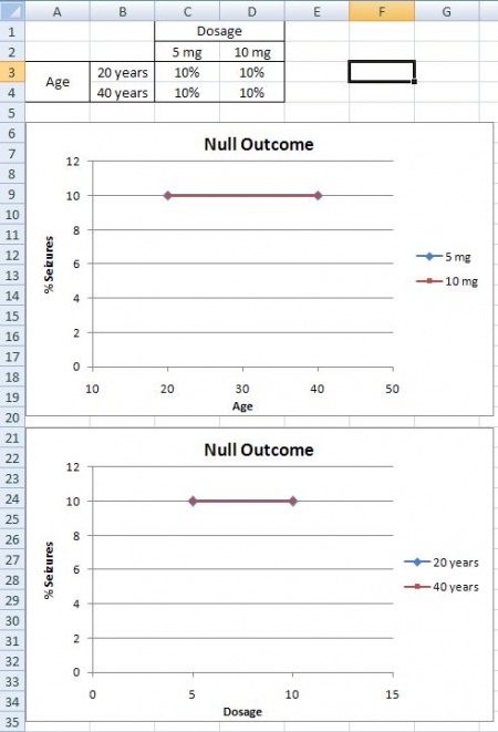
A null outcome situation is when the outcome of your experiment is the same regardless of how the levels within your experiment were combined. From the example above, a null outcome would exist if you received the same percentage of seizures occurring in patients with varying dose and age. The graphs below illustrate no change in the percentage of seizures for all factors, so you can conclude that the chance of suffering from a seizure is not affected by the dosage of the drug or the age of the patient.

Main Effects

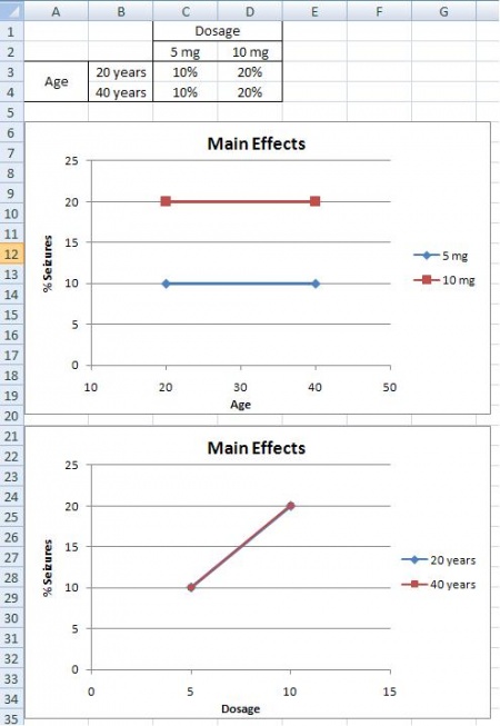
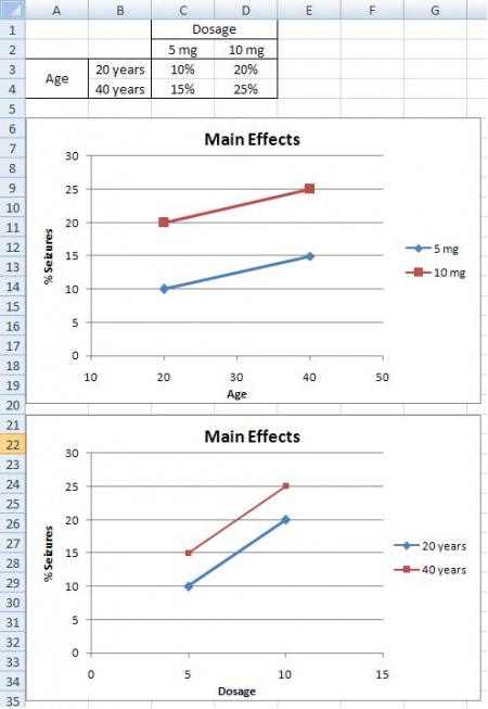
A main effects situation is when there exists a consistent trend among the different levels of a factor. From the example above, suppose you find that as dosage increases, the percentage of people who suffer from seizures increases as well. You also notice that age does not play a role; both 20 and 40 year olds suffer the same percentage of seizures for a given amount of CureAll. From this information, you can conclude that the chance of a patient suffering a seizure is minimized at lower dosages of the drug (5 mg). The second graph illustrates that with increased drug dosage there is an increased percentage of seizures, while the first graph illustrates that with increased age there is no change in the percentage of seizures. Both of these graphs only contain one main effect, since only dose has an effect the percentage of seizures. Whereas, graphs three and four have two main effects, since dose and age both have an effect on the percentage of seizures.

Interaction Effects

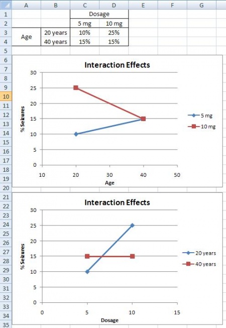
The interaction effects situation is the last outcome that can be detected using factorial design. From the example above, suppose you find that 20 year olds will suffer from seizures 10% of the time when given a 5 mg CureAll pill, while 20 year olds will suffer 25% of the time when given a 10 mg CureAll pill. When 40 year olds, however, are given a 5 mg pill or a 10 mg pill, 15% suffer from seizures at both of these dosages. This correlation can be seen in the graphs below. There is an increasing chance of suffering from a seizure at higher doses for 20 year olds, but no difference in suffering from seizures for 40 year olds. Thus, there must be an interaction effect between the dosage of CureAll, and the age of the patient taking the drug. When you have an interaction effect it is impossible to describe your results accurately without mentioning both factors. You can always spot an interaction in the graphs because when there are lines that are not parallel an interaction is present. If you observe the main effect graphs above, you will notice that all of the lines within a graph are parallel. In contrast, for interaction effect graphs, you will see that the lines are not parallel.

Mathematical Analysis Approach

In the previous section, we looked at a qualitative approach to determining the effects of different factors using factorial design. Now we are going to shift gears and look at factorial design in a quantitative approach in order to determine how much influence the factors in an experiment have on the outcome.

How to Deal with a 2ⁿ Factorial Design

Suppose you have two variables \(A\) and \(B\) and each have two levels a₁, a₂ and b₁, b₂. You would measure combination effects of \(A\) and \(B\) (a₁b₁, a₁b₂, a₂b₁, a₂b₂). Since we have two factors, each of which has two levels, we say that we have a 2 x 2 or a 2² factorial design. Typically, when performing factorial design, there will be two levels, and n different factors. Thus, the general form of factorial design is 2ⁿ.

In order to find the main effect of \(A\), we use the following equation:

\[A = (a_2b_1 - a_1b_1) + (a_2b_2 - a_1b_2) \nonumber \]

Similarly, the main effect of B is given by:

\[B = (b_2a_1 - b_1a_1) + (b_2a_2 - b_1a_2) \nonumber \]

By the traditional experimentation, each experiment would have to be isolated separately to fully find the effect on B. This would have resulted in 8 different experiments being performed. Note that only four experiments were required in factorial designs to solve for the eight values in A and B. This shows how factorial design is a timesaver.

By taking the coefficients in A and B, the table below was created.

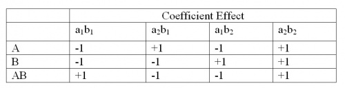
AB is found by multiplying the coefficients of a_xb_x to get the new coefficient effect.

The additional complication is the fact that more than one trial/replication is required for accuracy, so this requires adding up each sub-effect (e.g adding up the three trials of a₁b₁). By adding up the coefficient effects with the sub-effects (multiply coefficient with sub-effect), a total factorial effect can be found. This value will determine if the factor has a significant effect on the outcome. For larger numbers, the factor can be considered extremely important and for smaller numbers, the factor can be considered less important. The sign of the number also has a direct correlation to the effect being positive or negative.

To get a mean factorial effect, the totals needs to be divided by 2 times the number of replicates, where a replicate is a repeated experiment.

\[\text {mean factorial effect} = \dfrac{\text{total factorial effect}}{2r} \nonumber \]

By adding a third variable (\(C\)), the process of obtaining the coefficients becomes significantly complicated. The main factorial effect for \(A\):

\[A=\left(a_{2} b_{1} c_{1}-a_{1} b_{1} c_{1}\right)+\left(a_{2} b_{2} c_{1}-a_{1} b_{2} c_{1}\right)+\left(a_{2} b_{1} c_{2}-a_{1} b_{1} c_{2}\right)+\left(a_{2} b_{2} c_{2}-a_{1} b_{2} c_{2}\right) \nonumber \]

The table of coefficients is listed below

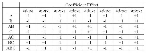
It is clear that in order to find the total factorial effects, you would have to find the main effects of the variable and then the coefficients. Yates Algorithm can be used to simplify the process.

Yates Algorithm

Frank Yates created an algorithm to easily find the total factorial effects in a 2ⁿ factorial that is easily programmable in Excel. While this algorithm is fairly straightforward, it is also quite tedious and is limited to 2ⁿ factorial designs. Thus, modern technology has allowed for this analysis to be done using statistical software programs through regression.

Steps:

1. In the first column, list all the individual experimental combinations

According to the yates order, such as follows for a 2³ factorial design

- - -

+ - -

- + -

+ + -

- - +

+ - +

- + +

+ + +

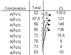
2. In the second column, list all the totals for each combination
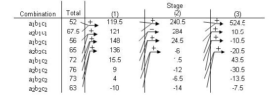
3. The 1^st four entries in the third column (Stage 1) are obtained by adding pairs together from the "totals list" (previous column). The next four numbers are obtained by subtracting the top number from the bottom number of each pair.

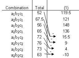
4. The fourth column (Stage 2) is obtained in the same fashion, but this time adding and subtracting pairs from Stage 1.

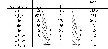
5. The fifth column (Stage 3) is obtained in the same fashion, but this time adding and subtracting pairs from Stage 2.

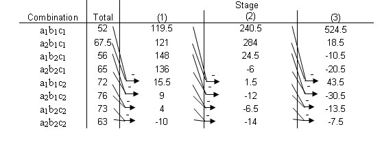
6. Continue with Stages until reaching n, or the number of factors. This final column is the Effect Total. A positive value means a positive correlation, and a negative values means a negative correlation. These values are all relative, however, so there is no way to compare different effect totals from different experiments.

Ignoring the first row, look in the last stage and find the variable that has the largest relative number, then that row indicates the MAIN TOTAL EFFECT. The Main Total Effect can be related to input variables by moving along the row and looking at the first column. If the row in the first column is a₂b₁c₁ then the main total effect is A. The row for a₁b₂c₁ would be for B. The row for a₂b₁c₂ would be for AC.

This main total effect value for each variable or variable combination will be some value that signifies the relationship between the output and the variable. For instance, if your value is positive, then there is a positive relationship between the variable and the output (i.e. as you increase the variable, the output increases as well). A negative value would signify a negative relationship. Notice, however, that the values are all relative to one another. So while the largest main total effect value in one set of experiments may have a value of 128, another experiment may have its largest main total effect value be 43. There is no way to determine if a value of 128 in one experiment has more control over its output than a value of 43 does, but for the purposes of comparing variables within an experiment, the main total effect does allow you to see the relative control the variables have on the output.

Factorial Design Example Revisited

Recall the example given in the previous section What is Factorial Design? In the example, there were two factors and two levels, which gave a 2² factorial design. The Yates Algorithm can be used in order to quantitatively determine which factor affects the percentage of seizures the most. For the use of the Yates algorithm, we will call age factor A with a₁ = 20 years, and a₂ = 40 years. Likewise, we will call dosage factor B, with b₁ = 5 mg, and b₂ = 10 mg. The data for the three outcomes is taken from the figures given in the example, assuming that the data given resulted from multiple trials.

Null Outcome

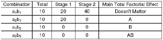
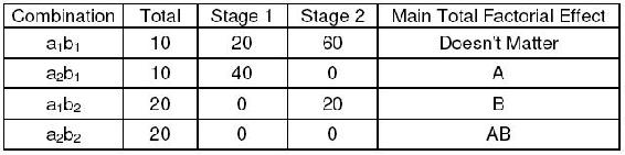
The following Yates algorithm table using the data for the null outcome was constructed. As seen in the table, the values of the main total factorial effect are 0 for A, B, and AB. This proves that neither dosage or age have any effect on percentage of seizures.

Main Effect

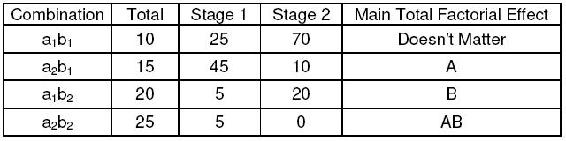
The following Yates algorithm table using the data from the first two graphs of the main effects section was constructed. Besides the first row in the table, the row with the largest main total factorial effect is the B row, while the main total effect for A is 0. This means that dosage (factor B) affects the percentage of seizures, while age (factor A) has no effect, which is also what was seen graphically.

The following Yates algorithm table using the data from second two graphs of the main effects section was constructed. Besides the first row in the table, the main total effect value was 10 for factor A and 20 for factor B. This means that both age and dosage affect percentage seizures. However, since the value for B is larger, dosage has a larger effect on percentage of seizures than age. This is what was seen graphically, since the graph with dosage on the horizontal axis has a slope with larger magnitude than the graph with age on the horizontal axis.

Interaction Effect

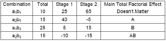
The following Yates algorithm table was constructed using the data from the interaction effects section. Since the main total factorial effect for AB is non-zero, there are interaction effects. This means that it is impossible to correlate the results with either one factor or another; both factors must be taken into account.

Chemical Engineering Applications

It should be quite clear that factorial design can be easily integrated into a chemical engineering application. Many chemical engineers face problems at their jobs when dealing with how to determine the effects of various factors on their outputs. For example, suppose that you have a reactor and want to study the effect of temperature, concentration and pressure on multiple outputs. In order to minimize the number of experiments that you would have to perform, you can utilize factorial design. This will allow you to determine the effects of temperature and pressure while saving money on performing unnecessary experiments.

A 2007 study on converting wheat straw to fuel utilized factorial design to study the effect of four factors on the composition and susceptibility to enzyme hydrolysis of the final product. (Perez, et.al.). The table below shows the full factorial design for the study. The four factors that were studied all had only two levels and dealt with pretreatment parameters. They were: Water temperature, residence time, solid fraction and overpressure in the reactor. It is not necessary to understand what each of these are to understand the experimental design. As seen in the table below, there were sixteen trials, or 2^4 experiments.

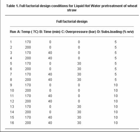
Source: Perez, et. al.

Minitab DOE Example

Minitab 15 Statistical Software is a powerful statistics program capable of performing regressions, ANOVA, control charts, DOE, and much more. Minitab is especially useful for creating and analyzing the results for DOE studies. It is possible to create factorial, response surface, mixture, and taguchi method DOEs in Minitab. The general method for creating factorial DOEs is discussed below.

Creating Factorial DOE

Minitab provides a simple and user-friendly method to design a table of experiments. Additionally, analysis of multiple responses (results obtained from experimentation) to determine which parameters significantly affect the responses is easy to do with Minitab. Minitab 15 Statistical Software can be used via Virtual CAEN Labs by going to Start>All Programs>Math and Numerical Methods>Minitab Solutions>Minitab 15 Statistical Software.

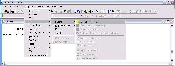
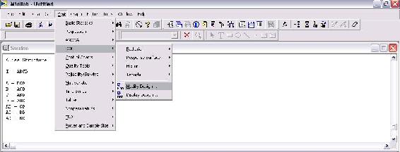
The first step is creating the DOE by specifying the number of levels (typically 2) and number of responses. To do this, go to Stat>DOE>Factorial>Create Factorial Design as shown in the image below.

The next image is the "Create Factorial Design" options menu.

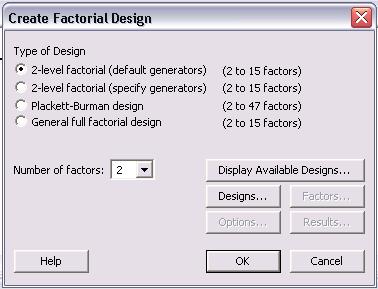
For a 2 level design, click the "2-level factorial (default generators)" radio button. Then specify the number of factors between 2 and 15. Other designs such as Plackett-Burman or a General full factorial design can be chosen. For information about these designs, please refer to the "Help" menu.

After the number of factors is chosen, click on the "Designs..." option to see the following menu.

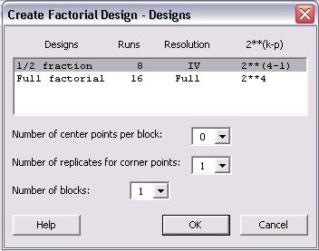
In this menu, a 1/2 fraction or full factorial design can be chosen. Although the full factorial provides better resolution and is a more complete analysis, the 1/2 fraction requires half the number of runs as the full factorial design. In lack of time or to get a general idea of the relationships, the 1/2 fraction design is a good choice. Additionally, the number of center points per block, number of replicates for corner points, and number of blocks can be chosen in this menu. Consult the "Help" menu for details about these options. Click "Ok" once the type of design has been chosen.

Once the design has been chosen, the "Factors...", "Options..." and "Results..." buttons become active in the "Create Factorial Designs" option menu. Click on "Factors..." button to see the following menu.

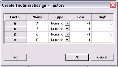
The above image is for a 4 factor design. Factors A - D can be renamed to represent the actual factors of the system. The factors can be numeric or text. Additionally, a low and high value are initially listed as -1 and 1, where -1 is the low and 1 is the high value. The low and high levels for each factor can be changed to their actual values in this menu. Click "OK" once this is completed.

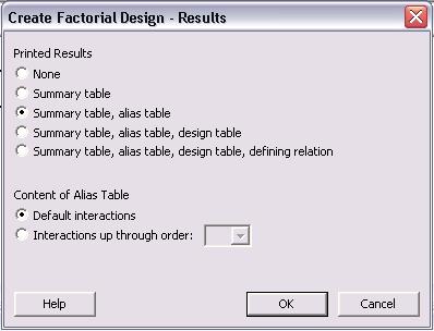
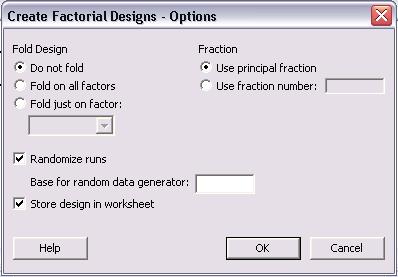
The necessary steps for creating the DOE are complete, but other options for "Results..." and "Options..." can be specified. The menus for "Results..." and "Options..." are shown below.

In the main "Create Factorial Design" menu, click "OK" once all specifications are complete. The following table is obtained for a 2-level, 4 factor, full factorial design. None of the levels were specified as they appear as -1 and 1 for low and high levels, respectively.

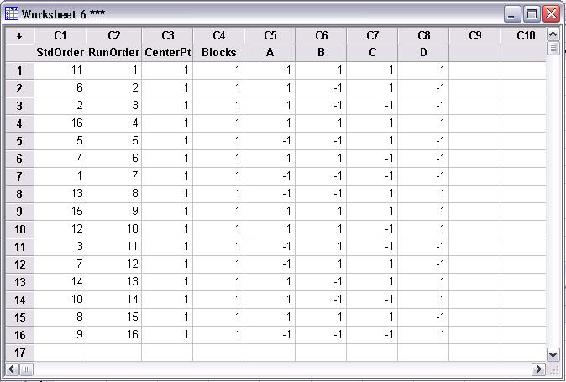
The above table contains all the conditions required for a full factorial DOE. Minitab displays the standard order and randomized run order in columns C1 and C2, respectively. Columns A-D are the factors. The first run (as specified by the random run order) should be performed at the low levels of A and C and the high levels of B and D. A total of 16 runs are required to complete the DOE.

Modifying DOE Table

Once a table of trials for the DOE has been created, additional modifications can be made as needed. Some typical modifications include modifying the name of each factors, specifying the high and low level of each factor, and adding replicates to the design. To being modifications of a current design, go to Stat>DOE>Modify Design... as seen in the figure below.

The following menu is displayed for modifying the design.

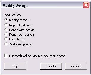
In the "Modify Design" menu, users can modify factors, replicate design, randomize design, renumber design, fold design, and add axial points. Additionally, any changes made can be put into a new worksheet. To change the factors, click the "Modify factors" radio button and then "Specify" to see the following options menu.

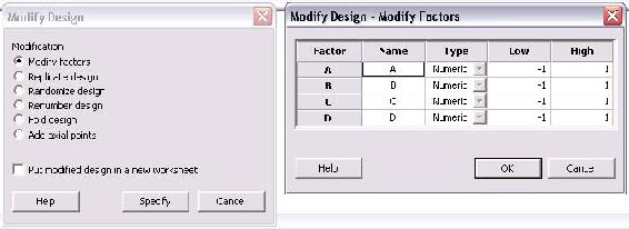
The default factors are named "A", "B", "C", and "D" and have respective high and low levels of 1 and -1. The name of the factors can be changed by simply clicking in the box and typing a new name. Additionally, the low and high levels for each factor can be modified in this menu. Since the high and low levels for each factor may not be known when the design is first created, it is convenient to be able to define them later. Click "OK" after modifications are complete.

Another typical modification is adding replicates to a design. Replicates are repeats of each trial that help determine the reproducibility of the design, thus increasing the number of trials and accuracy of the DOE. To add replicates, click the "Replicate design" radio button in the "Modify Design" menu. The following menu will be displayed.

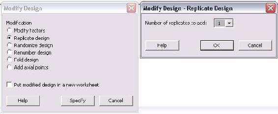
The only option in this menu is the number of replicates to add. The number ranges between 1 and 10. To have a total of 3 trials of each, the user should add 2 replicates in this menu. If 4 replicates are added, there will be a total of 5 trials of each. Typically, if the same experimentation will occur for 3 lab periods, 2 replicates will be added.

Additional modifications to the design include randomizing and renumbering the design. These are very straightforward modifications which affect the ordering of the trials. For information about the "Fold design" and "Add axial points", consult the "Help" menu.

Analyzing DOE Results

After the complete DOE study has been performed, Minitab can be used to analyze the effect of experimental results (referred to as responses) on the factors specified in the design. The first step in analyzing the results is entering the responses into the DOE table. This is done much like adding data into an Excel data sheet. In the columns to the right of the last factor, enter each response as seen in the figure below.

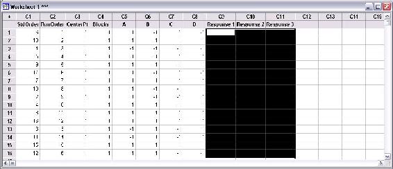
The above figure contains three response columns. The names of each response can be changed by clicking on the column name and entering the desired name. In the figure, the area selected in black is where the responses will be inputted. For instance, if the purity, yield, and residual amount of catalyst was measured in the DOE study, the values of these for each trial would be entered in the columns.

Once the responses are entered, statistical analysis on the data can be performed. Go to Stat>DOE>Factorial>Analyze Factorial Design... as seen in the following image.

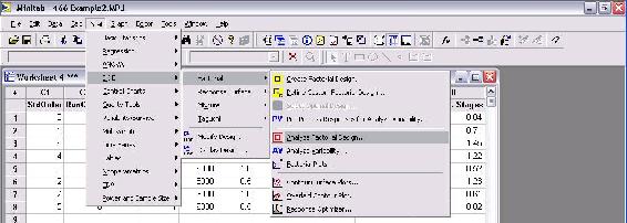
The menu that appears for analyzing factorial design is shown below.

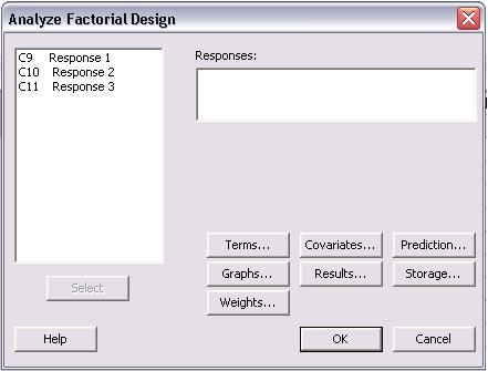
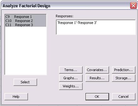
In the "Analyze Factorial Design" menu, the responses are shown on the left of the screen. The first step is to choose the responses to be analyzed. All of the responses can be chosen at once or individually. To choose them, click (or click and drag to select many) and then click "Select" to add them into the "Responses:" section as seen below.

The next step is selecting which terms will be analyzed for the responses. To do this, click on "Terms..." and the following menu will appear.

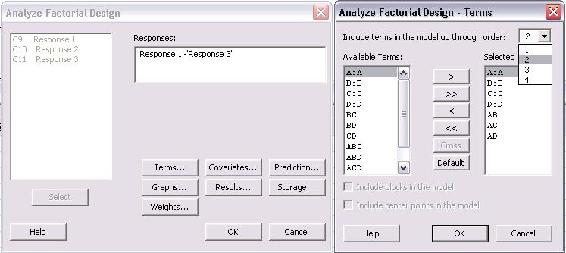
The types of interactions between factors are chosen in this menu. For a first order model which excludes all factor-to-factor interactions, "1" should be chosen from the drop-down menu for "Include terms in the model up through order:". To include higher order terms and account for factor interactions, choose 2, 3, or 4 from the drop-down menu. Unless significant factor-to-factor interactions are expected, it is recommended to use a first order model which is a linear approximation.

Once the terms have been chosen, the next step is determining which graphs should be created. The types of graphs can be selected by clicking on "Graphs..." in the main "Analyze Factorial Design" menu.

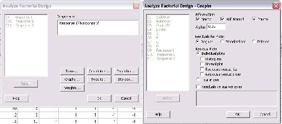
In the Graphs menu shown above, the three effects plots for "Normal", "Half Normal", and "Pareto" were selected. These plots are different ways to present the statistical results of the analysis. Examples of these plots can be found in the Minitab Example for Centrifugal Contactor Analysis. The alpha value, which determines the limit of statistical significance, can be chosen in this menu also. Typically, the alpha value is 0.05. The last type of plots that can be chosen is residual plots. A common one to select is "Residuals versus fits" which shows how the variance between the predicted values from the model and the actual values.

The final option that must be specified is results. Click "Results..." from the "Analyze Factorial Design" menu to see the following screen.

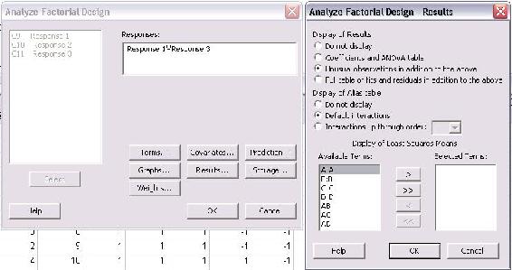
In this menu, select all of the "Available Terms" and click the ">>" button to move them to the "Selected Terms". This will ensure that all the terms will be included in the analysis. Another feature that can be selected from this menu is to display the "Coefficients and ANOVA table" for the DOE study.

Other options can be selected from the "Analyze Factorial Design" menu such as "Covariates...", "Prediction...", "Storage...", and "Weights...". Consult the "Help" menu for descriptions of the other options. Once all desired changes have been made, click "OK" to perform the analysis. All of the plots will pop-up on the screen and a text file of the results will be generated in the session file.

Minitab Example for Centrifugal Contactor Analysis

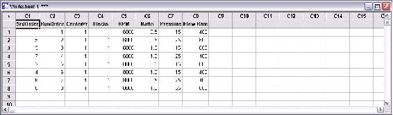
Centrifugal Contactors, also known as Podbielniak (POD) centrifugal contactors, are used to purify a contaminated stream by counter-current, liquid-liquid extraction. Two immiscible fluids with different specific gravities are contacted counter-currently and the solute from the dirty stream is extracted by the clean stream. A common use for PODs methanol removal from biodiesel by contacting the stream with water. The amount of methanol remaining in the biodiesel (wt% MeOH) after the purification and the number of theoretical stages (No. Theor. Stages) obtained depend on the operating conditions of the POD. The four main operating parameters of the POD are rotational speed (RPM), ratio of biodiesel to water (Ratio), total flow rate of biodiesel and water (Flow Rate), and pressure (Pressure). A DOE study has been performed to determine the effect of the four operating conditions on the responses of wt% MeOH in biodiesel and number of theoretical stages achieved. (NOTE: The actual data for this example was made-up)

A 4-factor, 2-level DOE study was created using Minitab. Because experiments from the POD are time consuming, a half fraction design of 8 trial was used. The figure below contains the table of trials for the DOE.

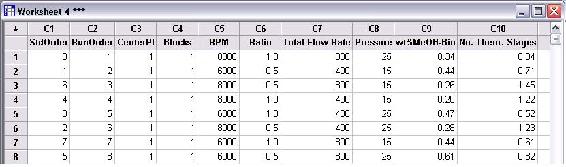
After all the trials were performed, the wt% methanol remaining in the biodiesel and number of theoretical stages achieved were calculated. The figure below contains the DOE table of trials including the two responses.

Analysis was performed on the DOE study to determine the effects of each factor on the responses. Only first order terms were included in the analysis to create a linear model. Pareto charts for both wt% MeOH in biodiesel and number of theoretical stages are shown below.

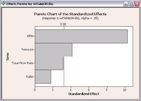
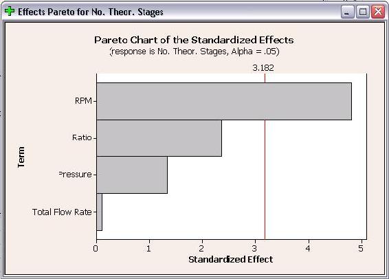
The Pareto charts show which factors have statistically significant effects on the responses. As seen in the above plots, RPM has significant effects for both responses and pressure has a statistically significant effect on wt% methanol in biodiesel. Neither flow rate or ratio have statistically significant effects on either response. The Pareto charts are bar charts which allow users to easily see which factors have significant effects.

Half Normal Plots for wt% methanol in biodiesel and number of theoretical stages are shown below.

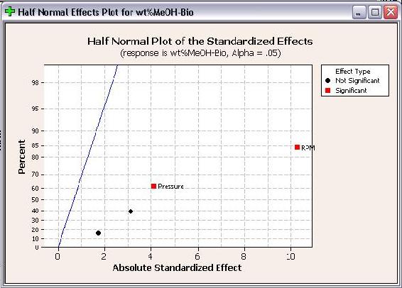
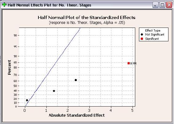
Like Pareto plots, Half Normal plots show which factors have significant effects on the responses. The factors that have significant effects are shown in red and the ones without significant effects are shown in black. The further a factor is from the blue line, the more significant effect it has on the corresponding response. For wt% methanol in biodiesel, RPM is further from the blue line than pressure, which indicates that RPM has a more significant effect on wt% methanol in biodiesel than pressure does.

The final plot created is the Normal Effect Plot. The Normal Plot is similar to the Half Normal plot in design. However, the Normal Plot displays whether the effect of the factor is positive or negative on the response. The Normal Plots for the responses are shown below.

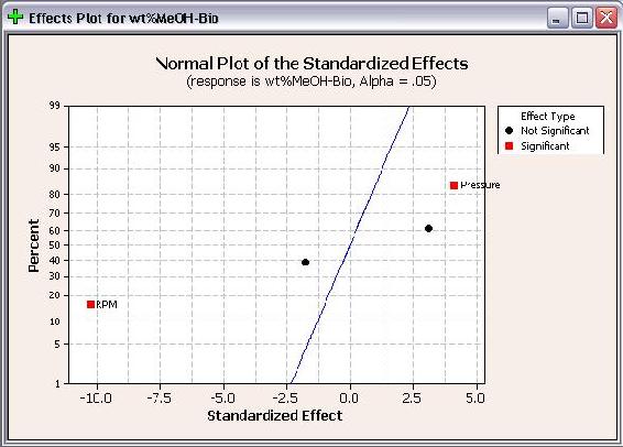
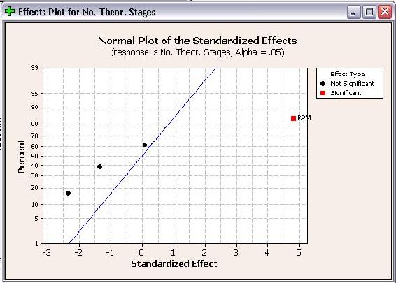
As seen above, RPM is shown with a positive effect for number of theoretical stages, but a negative effect for wt% methanol in biodiesel. A positive effect means that as RPM increases, the number of theoretical stages increases. Whereas a negative effect indicates that as RPM increases, the wt% methanol in biodiesel decreases. Fortunately for operation with the POD, these are desired results. When choosing operating conditions for the POD, RPM should be maximized to minimize the residual methanol in biodiesel and maximize the number of theoretical stages achieved.

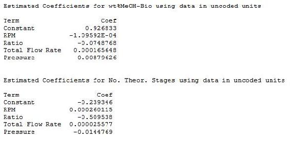
In addition to the above effects plots, Minitab calculates the coefficients and constants for response equations. The response equations can be used as models for predicting responses at different operating conditions (factors). The coefficients and constants for wt% methanol in biodiesel and number of theoretical stages are shown below.

Since this is a first order, linear model, the coefficients can be combined with the operating parameters to determine equations. The equations from this model are shown below.

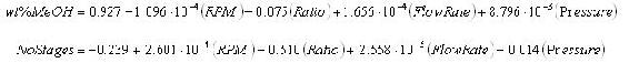
These equations can be used as a predictive model to determine wt% methanol in biodiesel and number of theoretical stages achieved at different operating conditions without actually performing the experiments. However, the limits of the model should be tested before the model is used to predict responses at many different operating conditions.

Example \(\PageIndex{1}\)

You have been employed by SuperGym, a local personal training gym, who want an engineer's perspective on how to offer the best plans to their clients. SuperGym currently categorizes her clients into 4 body types to help plan for the best possible program.

• Type 1 - Very healthy
• Type 2 - Needs tone
• Type 3 - Needs strength
• Type 4 - Needs tone and strength

In addition, SuperGym offers 4 different workout plans, A through D, none of which are directly catered to any of the different types. Create an experimental factorial design that could be used to test the effects of the different workout plans on the different types of people at the gym.

Solution

In order to solve this problem, we need to determine how many different experiments would need to be performed. In order to solve this, we can see that we have two different factors, body type and workout plan. For each factor, there exist four different levels. Thus, we have a 4² factorial design, which gives us 16 different experimental groups. Creating a table of all of the different groups, we arrive at the following factorial design:

Solution

A1	B1	C1	D1
A2	B2	C2	D2
A3	B3	C3	D3
A4	B4	C4	D4

Where A-D is the workout plan and 1-4 is the types

Example \(\PageIndex{2}\)

Suppose that you are looking to study the effects of hours slept (A), hours spent with significant other (B), and hours spent studying (C) on a students exam scores. You are given the following table that relates the combination of these factors and the students scores over the course of a semester. Use the Yates method in order to determine the effect each variable on the students performance in the course.

Given Information

1	17	24	19	21	22	28	25	24
2	18.5	21	20	19	26	22	27	19
3	16.5	22.5	22	25	24	26	21	20
Total	52	67.5	61	65	72	76	73	63

Solution

Using the approach introduced earlier in this article, we arrive at the following Yates solution.

			Stage		Main Total
Combination	Total	1	2	3	Factorial Effect
a1b1c1	52	119.5	245.5	529.9	Doesn't matter
a2b1c1	67.5	126	284	13.5	A
a1b2c1	61	148	19.5	-5.5	B
a2b2c1	65	136	-6	-25.5	AB
a1b1c2	72	15.5	6.5	38.5	C
a2b1c2	76	4	-12	-25.5	AC
a1b2c2	73	4	-11.5	-18.5	BC
a2b2c2	63	-10	-14	-2.5	ABC

From this table, we can see that there is positive correlation for factors A and C, meaning that more sleep and more studying leads to a better test grade in the class. Factor B, however, has a negative effect, which means that spending time with your significant other leads to a worse test score. The lesson here, therefore, is to spend more time sleeping and studying, and less time with your boyfriend or girlfriend.

Example \(\PageIndex{3}\)

Your mom is growing a garden for the state fair and has done some experiments to find the ideal growing condition for her vegetables. She asks you for help interpreting the results and shows you the following data:

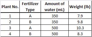
Make plots to determine the main or interaction effects of each factor.

Solution

Here is the plot you should have gotten for the given data.

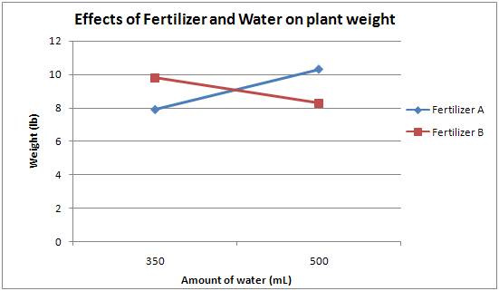
From this one can see that there is an interaction effect since the lines cross. One cannot discuss the results without speaking about both the type of fertilizer and the amount of water used. Using fertilizer A and 500 mL of water resulted in the largest plant, while fertilizer A and 350 mL gave the smallest plant. Fertilizer B and 350 mL gave the second largest plant, and fertilizer B and 500 mL gave the second smallest plant. There is clearly an interaction due to the amount of water used and the fertilizer present. Perhaps each fertilizer is most effective with a certain amount of water. In any case, your mom has to consider both the fertilizer type and amount of water provided to the plants when determining the proper growing conditions.

Exercise \(\PageIndex{1}\)

Which of the following is not an advantage of the use of factorial design over one factor design?

1. More time efficient
2. Provides how each factor effects the response
3. Does not require explicit testing
4. Does not require regression

Answer

TBA

Exercise \(\PageIndex{2}\)

In a 2² factorial design experiment, a total main effect value of -5 is obtained. This means that

1. there is a relative positive correlation between the two factors
2. there is no correlation between the two factors
3. there is a relative negative correlation between the two factors
4. there is either a positive or negative relative correlation between the two factors

Answer

TBA

References

• Box, George E.P., et. al. "Statistics for Engineers: An Introduction to Design, Data Analysis, and Model Building." New York: John Wiley & Sons.
• Trochim, William M.K. 2006. "Factorial Designs." Research Methods Knowledge Base. <http://www.socialresearchmethods.net/kb/expfact.htm>
• Perez, Jose A., et. al. "Effect of process variables on liquid hot water pretreatment of wheat straw for bioconversion to fuel-ethanol in a batch reactor." Journal of Chemical Technology & Biotechnology. Volume 82, Issue 10, Pages 929-938. Published Online Sep 3, 2007.