9.3: Hydraulic jumps and bores

Figure \(\PageIndex{1}\): A hydraulic jump downstream of a constriction. The jump is enclosed by the region \(x_u\) < x < \(x_d\). Upstream and downstream flows have velocity and depth equal to {\(u_u\),H},{\(u_d\),rH}.

Figure \(\PageIndex{2}\): Based on the traditional nursery rhyme Fleas, Lewis Fry Richardson’s tongue-in-cheek description of the turbulent energy cascade is both poetic and accurate. The “whorls” shown here, both big and little, were generated by the Colbuco volcano in Chile, photographed by Marcelo Reyes. Richardson, 1881-1953, was an English mathematician and psychologist. He invented the first algorithms for numerical weather forecasting decades before there were computers to execute them. He was also a dedicated pacifist and published important statistical studies on the causation and prevention of wars.

9.3.1 A stationary hydraulic jump in a rectilinear channel

Downstream of a hydraulic control, the supercritical flow state is unstable. As a result it becomes turbulent and returns to a subcritical state (slower, deeper flow). This transition is called a hydraulic jump. As the name suggests, it can be quite sudden (Figure \(\PageIndex{1}\)).

The hydraulic jump is a situation where we cannot ignore turbulence, but we will model its effects in the simplest way possible. The effect of turbulence on a unidirectional channel flow is to divert some of the mean downstream motion into chaotic swirls and eddies. These motions carry no net momentum (the swirling motion is as likely to go in one direction as another), but they do carry kinetic energy. Energy diverted into turbulence does not usually return to the mean flow. Instead, it is converted into progressively smaller eddies (e.g., Figures 5.3.4, \(\PageIndex{2}\)) and ultimately converted to internal energy via frictional dissipation (sections 6.4.2, 6.4.3).

Our goals here are to make testable predictions of the downstream flow state. Is it deeper or shallower than upstream? Slower or faster? And by how much? Our tools will be the familiar equations of momentum and mass conservation plus a new energy conservation law that accounts for turbulence.

To simplify the analysis, we return to the case of a rectilinear channel. We retain the assumptions that the fluid is inviscid and homogeneous, and we assume further that, in the vicinity of the hydraulic jump, the bottom is flat (\(h\) = 0). The momentum and mass equations describing the mean flow are

\[u_{t}=-u u_{x}-g \eta_{x}\label{eqn:1} \]

\[\eta_{t}=-[u(H+\eta)]_{x}.\label{eqn:2} \]

Now consider the vertically-integrated streamwise momentum

\[M(x, t)=\int_{-H}^{\eta} u d z=u(\eta+H). \nonumber \]

The evolution of \(M\) is governed by:

\[\begin{aligned}
M_{t} &=u_{t}(\eta+H)+u \eta_{t} \\
&=\left(-u u_{x}-g \eta_{x}\right)(\eta+H)-u[u(H+\eta)]_{x} \\
&=-u_{x} u(\eta+H)-g(H+\eta)_{x}(\eta+H)-u[u(H+\eta)]_{x}.
\end{aligned} \nonumber \]

We have used the fact that \(\eta_x = (H +\eta)_x\), because \(H\) is constant. The first and third terms combine to form a complete derivative, as does the middle term:

\[M_{t}=-\left[u^{2}(\eta+H)\right]_{x}-g \frac{1}{2}\left[(H+\eta)^{2}\right]_{x}, \nonumber \]

or

\[M_{t}=-\mathscr{F}_{x}^{(m)}, \quad \text { where } \quad \mathscr{F}^{(m)}=u^{2}(\eta+H)+\frac{g}{2}(H+\eta)^{2}.\label{eqn:3} \]

This tells us that the vertically-integrated momentum is governed by the convergence of the momentum flux \(\mathscr{F}(m)\).

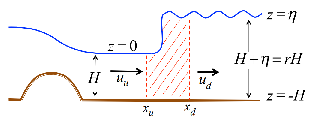
Now consider a steady hydraulic jump, as shown in Figure \(\PageIndex{1}\). Equations Equation \(\ref{eqn:2}\) and Equation \(\ref{eqn:3}\) provide two constraints that determine the change in depth and velocity across the jump. First, the mass flux exiting the jump must be the same as that entering it:

\[[u(H+\eta)]_{x_{u}}^{x_{d}}=0.\label{eqn:4} \]

Second, the momentum flux must be the same exiting as entering:

\[\left[u^{2}(\eta+H)+\frac{g}{2}(H+\eta)^{2}\right]_{x_{u}}^{x_{d}}=0.\label{eqn:5} \]

To apply these constraints, we first relabel the upstream and downstream velocities as \(u_u\) and \(u_d\) (see Figure \(\PageIndex{1}\)) . The upstream depth is \(H\) and the downstream depth is

\[H+\eta=r H, \nonumber \]

where the depth ratio \(r\) is a constant. If the flow deepens across the jump as shown in Figure \(\PageIndex{1}\), then \(r\) > 1. Substituting into Equation \(\ref{eqn:4}\) and Equation \(\ref{eqn:5}\),

\[u_{u} H=u_{d} r H,\label{eqn:6} \]

\[H u_{u}^{2}+\frac{g}{2} H^{2}=r H u_{d}^{2}+\frac{g}{2} r^{2} H^{2}.\label{eqn:7} \]

From Equation \(\ref{eqn:6}\), we have

\[u_{d}=\frac{u_{u}}{r}.\label{eqn:8} \]

Substituting this in Equation \(\ref{eqn:7}\) and cancelling a factor \(H\), we obtain

\[u_{u}^{2}+\frac{g}{2} H=\frac{u_{u}^{2}}{r}+\frac{g}{2} r^{2} H. \nonumber \]

This is easily solved for \(u_u\):

\[u_{u}=\sqrt{\frac{g H}{2} r(r+1)}.\label{eqn:9} \]

Using Equation \(\ref{eqn:8}\), we also have

\[u_{d}=\sqrt{\frac{g H}{2} \frac{r+1}{r}}.\label{eqn:10} \]

To predict the downstream flow state, assume that we know the upstream velocity \(u_u\) and depth \(H\), which gives the upstream Froude number:

\[F_{u}^{2}=\frac{u_{u}^{2}}{g H}=\frac{r(r+1)}{2}. \nonumber \]

This is a quadratic equation for \(r\) with a single positive solution:

\[r=\frac{\sqrt{1+8 F_{u}^{2}}-1}{2}.\label{eqn:11} \]

We are now able to predict both the downstream velocity \(u_d = u_u/r\) and the downstream depth \(rH\). To complete the picture we add the downstream Froude number:

\[F_{d}^{2}=\frac{u_{d}^{2}}{g(H+\eta)}=\frac{u_{u}^{2} / r^{2}}{g r H}=\frac{F_{u}^{2}}{r^{3}}=\frac{r+1}{2 r^{2}}. \nonumber \]

Example \(\PageIndex{1}\)

Consider a dam spillway with water depth \(H\) = 1 m and velocity \(u_u\) = 6 m/s. The Froude number is easily computed:

\[F_{u}=\frac{6 \mathrm{m} / \mathrm{s}}{\sqrt{9.8 \mathrm{m} / \mathrm{s}^{2} \times 1 \mathrm{m}}}=1.92. \nonumber \]

Because the flow is supercritical, we expect to see a hydraulic jump. From Equation \(\ref{eqn:11}\) we compute \(r\) = 2.26. The downstream flow is therefore slower and deeper, with depth \(rH\) = 2.26 m and velocity \(u_u/r\) = 2.65 m/s. The downstream Froude number is subcritical: \(F_d\) = \(F_u/r^{3/2}\) = 0.32.

An important question remains to be addressed. So far, we have assumed that \(r\) > 1, in which case

\[F_{u}^{2}=\frac{r(r+1)}{2}>1, \quad \text { and } \quad F_{d}^{2}=\frac{r+1}{2 r^{2}}<1. \nonumber \]

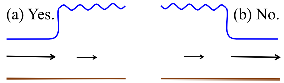
Now, suppose that \(r\) < 1. The results are opposite: \(F_u\) < 1 and \(F_d\) > 1, i.e., the transition is from a subcritical to a supercritical state, with flow becoming shallower and faster. This is a perfectly valid solution of the momentum and mass equations as developed above. Yet, it is a phenomenon never seen in nature (Figure \(\PageIndex{3}\)). Why? This paradox exists because we have not yet considered the conservation of energy.

Figure \(\PageIndex{3}\): Why do hydraulic jumps always look like (a), and never (b)?

9.3.2 Energy flux and the effects of turbulence

At a given location, the specific mechanical energy of the mean flow (kinetic plus potential, per unit mass) is \(\frac{1}{2}u^2 +gz\). Integrating this over the vertical extent of the flow, and remembering that \(u\) is independent of \(z\), we have

\[\begin{aligned}
E(x, t) &=\int_{-H}^{\eta}\left(\frac{1}{2} u^{2}+g z\right) d z \\
&=\left[\frac{1}{2} u^{2} z+\frac{1}{2} g z^{2}\right]_{-H}^{\eta} \\
&=\frac{1}{2} u^{2}(\eta+H)+\frac{1}{2} g\left(\eta^{2}-H^{2}\right).
\end{aligned} \nonumber \]

Our task now is to find the equation that governs \(E(x,t)\). Differentiating with respect to time, we obtain

\[E_{t}=u u_{t}(\eta+H)+\frac{1}{2} u^{2} \eta_{t}+g \eta \eta_{t}. \nonumber \]

Now from Equation 9.2.4,

\[u_{t}=-u u_{x}-g \eta_{x}=-\left(\frac{1}{2} u^{2}+g \eta\right)_{x} \nonumber \]

and from 9.2.11,

\[\eta_{t}=-\left(\frac{Q}{W}\right)_{x}, \nonumber \]

where \(Q/W = u(\eta +H)\). Substituting, we have

\[\begin{aligned}
E_{t} &=-u\left(\frac{1}{2} u^{2}+g \eta\right)_{x}(\eta+H)-\left(\frac{1}{2} u^{2}+g \eta\right)\left(\frac{Q}{W}\right)_{x} \\
&=-\frac{Q}{W}\left(\frac{1}{2} u^{2}+g \eta\right)_{x}-\left(\frac{Q}{W}\right)_{x}\left(\frac{1}{2} u^{2}+g \eta\right) \\
&=-\left[\frac{Q}{W}\left(\frac{1}{2} u^{2}+g \eta\right)\right]_{x},
\end{aligned} \nonumber \]

or

\[E_{t}=-\mathscr{F}_{x}^{(e)},\label{eqn:12} \]

in which

\[\mathscr{F}^{(e)}=\frac{Q}{W}\left(\frac{1}{2} u^{2}+g \eta\right) \nonumber \]

is the downstream flux of mechanical energy in the mean flow.

Now suppose we wanted to account for the fact that some mechanical energy is diverted into turbulent motions. The equations of motion would then include some very complicated additional terms, and Equation \(\ref{eqn:12}\) would take the form

\[E_{t}=-\mathscr{F}_{x}^{(e)}-\mathscr{E},\label{eqn:13} \]

where the new term \(\mathscr{E}\) represents the rate of energy loss to turbulence. Explicit calculation of \(\mathscr{E}\) is not practical. Happily, all we need to know here is that \(\mathscr{E}\) is positive, i.e., turbulent dissipation only works one way, and that is to reduce the mechanical energy of the flow.

In steady state, then, \(E_t\) = 0 and Equation \(\ref{eqn:13}\) becomes

\[\mathscr{F}_{x}^{(e)}=-\mathscr{E}<0. \nonumber \]

This inequality simply states that the flux of mechanical energy exiting a turbulent region is less than the flux entering it. To apply this to the hydraulic jump shown in Figure \(\PageIndex{1}\), we integrate from \(x_u\) to \(x_d\) and obtain

\[\int_{x_{u}}^{x_{d}} \mathscr{F}_{x}^{(e)} d x=\left.\mathscr{F}^{(e)}\right|_{x_{u}} ^{x_{d}}=\frac{Q}{W}\left(\frac{1}{2} u_{d}^{2}+g \eta-\frac{1}{2} u_{u}^{2}\right)<0. \nonumber \]

We have oriented our coordinates such that \(Q\) > 0, and therefore

\[\frac{1}{2} u_{d}^{2}+g \eta-\frac{1}{2} u_{u}^{2}<0. \nonumber \]

Substitution from Equation \(\ref{eqn:8}\), Equation \(\ref{eqn:9}\) and Equation \(\ref{eqn:11}\) gives

\[\frac{1}{2} \frac{g H}{2} \frac{r+1}{r}+g(r-1) H-\frac{1}{2} \frac{g H}{2} r(r+1)<0. \nonumber \]

With a little algebra, this becomes

\[(1-r)^{3}<0, \quad \text { therefore } \quad r>1. \nonumber \]

If \(r\) were less than 1, this condition would be violated, meaning that the mean flow would gain energy from the turbulence, an impossibility. As a result, hydraulic jumps in the real world always carry the flow from a supercritical to a subcritical state, as in Figure \(\PageIndex{3}\)a.

Figure \(\PageIndex{4}\): Definition sketch for velocities in (a) a stationary hydraulic jump (upper) and (b) a bore moving into still water (lower). The wave is the same; the only difference is the reference frame. The velocities \(u_u\) and \(u_d\) are given by Equation \(\ref{eqn:9}\) and Equation \(\ref{eqn:8}\).

Figure \(\PageIndex{5}\): Definition sketch for two-dimensional, free-surface flow in a tilted channel.

9.3.3 A hydraulic bore

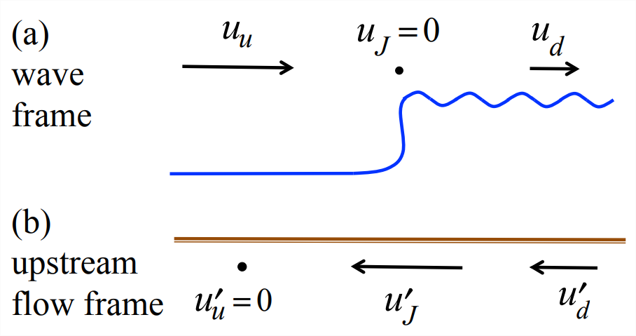
Until now we have assumed that our hydraulic jump is stationary, as it would be downstream of a fixed obstruction. A very similar phenomenon is a bore, which is basically a moving hydraulic jump. A good example is swash, i.e., a beach wave after it breaks.

Mathematical analysis requires only that we subtract the appropriate velocity from Equation \(\ref{eqn:8}\) and Equation \(\ref{eqn:9}\). In the stationary case considered previously, we have upstream velocity \(u_u\) and downstream velocity \(u_d\), while the velocity of the jump, which we will call \(u_J\), is zero (Figure \(\PageIndex{4}\)a). Now suppose the jump is moving into a quiescent region (Figure \(\PageIndex{4}\)b). To use our previous results, we subtract \(u_u\) from all velocities, so that the new upstream velocity \(u^\prime_u\) = 0. Similarly, the downstream velocity \(u^\prime_d\) = \(u_d −u_u\) and the jump velocity \(u^\prime_J\) = \(−u_u\), where \(u_u\) and \(u_d\) are still as given by Equation \(\ref{eqn:9}\) and Equation \(\ref{eqn:8}\).

Two features are worth noting:

• The bore propagates leftward relative to the upstream fluid at a velocity \[u_{J}^{\prime}=-u_{u}=-\sqrt{\frac{g H}{2} r(r+1)}.\label{eqn:14} \] Its speed is then \[\left|u_{J}^{\prime}\right|=\sqrt{g H r} \sqrt{\frac{(r+1)}{2}}>\sqrt{g H r} \text { for } r>1. \nonumber \] This speed is greater than the linear long wave speed, the “speed limit” for small-amplitude waves. This is an example of nonlinear speedup, the tendency for nonlinear effects to increase the speed of a disturbance. The greater the height of the bore (i.e., r), the greater the speedup.
• The flow behind the bore moves to the left with speed \[\left|u_{d}^{\prime}\right|=\left|u_{d}-u_{u}\right|=\sqrt{\frac{g H}{2} r(r+1)}\left(1-\frac{1}{r}\right)<\sqrt{\frac{g H}{2} r(r+1)} \nonumber \] This means that the current behind the bore moves more slowly than the bore itself. More specifically, the ratio of the speed of the water behind the bore to that of the bore itself is \[\frac{u_{d}^{\prime}}{u_{J}^{\prime}}=1-\frac{1}{r}. \nonumber \] Two limiting cases are of interest:
  • In the limit \(r\rightarrow 1\), the water behind the bore is nearly stationary (\(u^\prime_d\rightarrow 0\)). This is similar to the case of small-amplitude waves, where the surrounding water does not travel with the wave.
  • In the limit \(r \rightarrow \inf\), \(u^\prime_d \rightarrow u^\prime_J\), i.e. when a large bore travels into shallow water, it becomes a “wall of water”, traveling almost as a solid object.

In some cases, both the bore and the upstream water are moving, e.g., a tidal bore advancing up a river. In that case, Equation \(\ref{eqn:14}\) still gives the speed of the wave relative to the upstream flow that it is propagating into. If you know the speed of the upstream (or the downstream) flow, you can calculate the speed of the wave relative to the shore, or relative to any other reference frame that may be relevant.