1.7: Experiment #7: Osborne Reynolds' Demonstration

Last updated
Save as PDF

Page ID: 28398

$ \newcommand{\vecs}[1]{\overset { \scriptstyle \rightharpoonup} {\mathbf{#1}} } $ $ \newcommand{\vecd}[1]{\overset{-\!-\!\rightharpoonup}{\vphantom{a}\smash {#1}}} $$\newcommand{\id}{\mathrm{id}}$ $ \newcommand{\Span}{\mathrm{span}}$ $ \newcommand{\kernel}{\mathrm{null}\,}$ $ \newcommand{\range}{\mathrm{range}\,}$ $ \newcommand{\RealPart}{\mathrm{Re}}$ $ \newcommand{\ImaginaryPart}{\mathrm{Im}}$ $ \newcommand{\Argument}{\mathrm{Arg}}$ $ \newcommand{\norm}[1]{\| #1 \|}$ $ \newcommand{\inner}[2]{\langle #1, #2 \rangle}$ $ \newcommand{\Span}{\mathrm{span}}$ $\newcommand{\id}{\mathrm{id}}$ $ \newcommand{\Span}{\mathrm{span}}$ $ \newcommand{\kernel}{\mathrm{null}\,}$ $ \newcommand{\range}{\mathrm{range}\,}$ $ \newcommand{\RealPart}{\mathrm{Re}}$ $ \newcommand{\ImaginaryPart}{\mathrm{Im}}$ $ \newcommand{\Argument}{\mathrm{Arg}}$ $ \newcommand{\norm}[1]{\| #1 \|}$ $ \newcommand{\inner}[2]{\langle #1, #2 \rangle}$ $ \newcommand{\Span}{\mathrm{span}}$$\newcommand{\AA}{\unicode[.8,0]{x212B}}$

1. Introduction

In nature and in laboratory experiments, flow may occur under two very different regimes: laminar and turbulent. In laminar flows, fluid particles move in layers, sliding over each other, causing a small energy exchange to occur between layers. Laminar flow occurs in fluids with high viscosity, moving at slow velocity. The turbulent flow, on the other hand, is characterized by random movements and intermixing of fluid particles, with a great exchange of energy throughout the fluid. This type of flow occurs in fluids with low viscosity and high velocity. The dimensionless Reynolds number is used to classify the state of flow. The Reynolds Number Demonstration is a classic experiment, based on visualizing flow behavior by slowly and steadily injecting dye into a pipe. This experiment was first performed by Osborne Reynolds in the late nineteenth century.

2. Practical Application

The Reynolds number has many practical applications, as it provides engineers with immediate information about the state of flow throughout pipes, streams, and soils, helping them apply the proper relationships to solve the problem at hand. It is also very useful for dimensional analysis and similitude. As an example, if forces acting on a ship need to be studied in the laboratory for design purposes, the Reynolds number of the flow acting on the model in the lab and on the prototype in the field should be the same.

3. Objective

The objective of this lab experiment is to illustrate laminar, transitional, and fully turbulent flows in a pipe, and to determine under which conditions each flow regime occurs.

4. Method

The visualization of flow behavior will be performed by slowly and steadily injecting dye into a pipe. The state of the flow (laminar, transitional, and turbulent) will be visually determined and compared with the results from the calculation of the Reynolds number.

5. Equipment

The following equipment is required to perform the Reynolds number experiment:

F1-10 hydraulics bench,
The F1-20 Reynolds demonstration apparatus,
Cylinder for measuring flow,
Stopwatch for timing the flow measurement, and
Thermometer.

6. Equipment Description

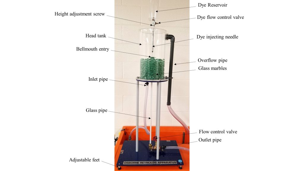
The equipment includes a vertical head tank that provides a constant head of water through a bellmouth entry to the flow visualization glass pipe. Stilling media (marbles) are placed inside the tank to tranquilize the flow of water entering the pipe. The discharge through this pipe is regulated by a control valve and can be measured using a measuring cylinder [7]. The flow velocity, therefore, can be determined to calculate Reynolds number. A dye reservoir is mounted on top of the head tank, from which a blue dye can be injected into the water to enable observation of flow conditions (Figure 7.1).

Diagram of Armfield F1-20 Reynolds apparatus. The top of the apparatus holds the dye reservoir which is connected to the head tank by a height adjustment screw. The dye flow control valve is connected to the side of the dye reservoir tube. The dye injecting needle extendes from the dye reservoir into the head tank just above the Bellmouth entry which rests atop a pile of glass marbles. At the top right side of the head tank, the overflow pipe which runs down to the base of the table. There is an inlet pipe and a glass pipe connected to the base of the head tank which run down to the base of the apparatus where the flow control valve and outlet pipe are located.

Figure 7.1: Armfield F1-20 Reynolds apparatus [7]

7. Theory

Flow behavior in natural or artificial systems depends on which forces (inertia, viscous, gravity, surface tension, etc.) predominate. In slow-moving laminar flows, viscous forces are dominant, and the fluid behaves as if the layers are sliding over each other. In turbulent flows, the flow behavior is chaotic and changes dramatically, since the inertial forces are more significant than the viscous forces.

In this experiment, the dye injected into a laminar flow will form a clear well-defined line. It will mix with the water only minimally, due to molecular diffusion. When the flow in the pipe is turbulent, the dye will rapidly mix with the water, due to the substantial lateral movement and energy exchange in the flow. There is also a transitional stage between laminar and turbulent flows, in which the dye stream will wander about and show intermittent bursts of mixing, followed by a more laminar behavior.

The Reynolds number (Re), provides a useful way of characterizing the flow. It is defined as:

$Re=\frac{vd} {\nu} \qquad (1)$

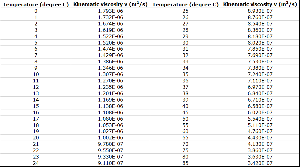
where ( $\nu$ ) is the kinematic viscosity of the water (Figure 7.2), v is the mean flow velocity and d is the diameter of the pipe.

The Reynolds number is a dimensionless parameter that is the ratio of the inertial (destabilizing) force to the viscosity (stabilizing) force. As Re increases, the inertial force becomes relatively larger, and the flow destabilizes and becomes fully turbulent.

The Reynolds experiment determines the critical Reynolds number for pipe flow at which laminar flow (Re<2000 ) becomes transitional (2000<Re<4000 ) and the transitional flow becomes turbulent (Re>4000). The advantage of using a critical Reynolds number, instead of critical velocity, is that the results of the experiments are applicable to all Newtonian fluid flows in pipes with a circular cross-section.

Table of Kinematic Viscosity of Water at Atmospheric Pressure. The first column displays temperature in degrees celsius from 0 to 24. The second column displays kinematic viscosity represented by v in meters squared per sec. The third column displays temperature in degrees celsius from 25 to 85. The fourth column displays kinematic viscosity represented by v in meters squared per sec.

Figure 7.2: Kinematic Viscosity of Water at Atmospheric Pressure.

8. Experimental Procedure

Thumbnail for the embedded element "Experiment # 7: Osborne Reynolds' Demonstration"

A YouTube element has been excluded from this version of the text. You can view it online here: https://uta.pressbooks.pub/appliedfluidmechanics/?p=237

Set up the equipment as follows:

Position the Reynolds apparatus on a fixed, vibration-free surface (not on the hydraulics bench), and ensure that the base is horizontal and the test section is vertical.
Connect the bench outflow to the head tank inlet pipe.
Place the head tank overflow tube in the volumetric tank of the hydraulics bench.
Attach a small tube to the apparatus flow control valve, and clamp it to a fixed position in a sink in the lab, allowing enough space below the end of the tube to insert a measuring cylinder. The outflow should not be returned to the volumetric tank since it contains dye and will taint the flow visualisation.

Note that any movement of the outflow tube during a test will cause changes in the flow rate, since it is driven by the height difference between the head tank surface and the outflow point.

Start the pump, slightly open the apparatus flow control valve and the bench valve, and allow the head tank to fill with water. Make sure that the flow visualisation pipe is properly filled. Once the water level in the head tank reaches the overflow tube, adjust the bench control valve to produce a low overflow rate.
Ensuring that the dye control valve is closed, add the blue dye to the dye reservoir until it is about 2/3 full.
Attach the needle, hold the dye assembly over a lab sink, and open the valve to ensure that there is a free flow of dye.
Close the dye control valve, then mount the dye injector on the head tank and lower the injector until the tip of the needle is slightly above the bellmouth and is centered on its axis.
Adjust the bench valve and flow control valve to return the overflow rate to a small amount, and allow the apparatus to stand for at least five minutes
Adjust the flow control valve to reach a slow trickle outflow, then adjust the dye control valve until a slow flow with clear dye indication is achieved.
Measure the flow volumetric rate by timed water collection.
Observe the flow patterns, take pictures, or make hand sketches as needed to classify the flow regime.
Increase the flow rate by opening the flow control valve. Repeat the experiment to visualize transitional flow and then, at higher flow rates, turbulent flow, as characterized by continuous and very rapid mixing of the dye. Try to observe each flow regime two or three times, for a total of eight readings.
As the flow rate increases, adjust the bench valve to keep the water level constant in the head tank.

Note that at intermediate flows, it is possible to have a laminar characteristic in the upper part of the test section, which develops into transitional flow lower down. This upper section behavior is described as an “inlet length flow,” which means that the boundary layer has not yet extended across the pipe radius.

Measure water temperature.
Return the remaining dye to the storage container. Rinse the dye reservoir thoroughly to ensure that no dye is left in the valve, injector, or needle.

9. Results and Calculations

Please visit this link for accessing excel workbook for this experiment.

The following dimensions of the equipment are used in the appropriate calculations. If required, measure them to make sure that they are accurate [7].

Diameter of test pipe: d = 0.010 m
Cross-sectional area of test pipe: A =7.854×10^-5m²

9.1. Results

Use the following table to record your measurements and observations.

Raw Data Table

Observed Flow Regime	Volume (L)	Time (sec)	Temperature ( $\circ_C$ )

9.2. Calculations

Calculate discharge, flow velocity, and Reynolds number ( Re). Classify the flow based on the Re of each experiment. Record your calculations in the following table.

Result Table

Observed Flow Regime	Discharge Q(m³/sec)	Velocity v(m/sec)	Kinematic Viscosity v(m²/s)	Renolds Number	Flow Regime Classified using Reynolds Number

10. Report

Use the template provided to prepare your lab report for this experiment. Your report should include the following:

Table(s) of raw data
Table(s) of results
A description, with illustrative sketches or photos, of the flow characteristics of each experimental run.
Discuss your results, focusing on the following:
- How is the flow pattern of each of the three states of flow (laminar, transitional, and turbulent) different?
- Does the observed flow condition occur within the expected Reynold’s number range for that condition?
Discuss your observation and any source of error in the calculation of the number.
Compare the experimental results with any theoretical studies you have undertaken.