4.4: Terminal Settling Velocity Equations

Stokes, Budryck and Rittinger used these drag coefficients to calculate settling velocities for laminar settling (Stokes), a transition zone (Budryck) and turbulent settling (Rittinger) of real sand grains. This gives the following equations for the settling velocity:

Laminar flow, d<0.1 mm, according to Stokes.

\[\ \mathrm{v}_{\mathrm{t}}=\mathrm{4 2 4} \cdot \mathrm{R}_{\mathrm{s} \mathrm{d}} \cdot \mathrm{d}^{\mathrm{2}}\]

Transition zone, d>0.1 mm and d<1 mm, according to Budryck.

\[\ \mathrm{v}_{\mathrm{t}}=\mathrm{8 . 9 2 5} \cdot \frac{(\sqrt{\left(\mathrm{1 + 9 5} \cdot \mathrm{R}_{\mathrm{s d}} \cdot \mathrm{d}^{3}\right)}-\mathrm{1})}{\mathrm{d}}\]

Turbulent flow, d>1 mm, according to Rittinger.

\[\ \mathrm{v}_{\mathrm{t}}=\mathrm{8 7} \cdot \sqrt{\mathrm{R}_{\mathrm{s} \mathrm{d}} \cdot \mathrm{d}}\]

With the relative submerged density R_sd defined as:

\[\ \mathrm{\mathrm{R}_{\mathrm{sd}}=\frac{\rho_{\mathrm{s}}-\rho_{\mathrm{l}}}{\rho_{\mathrm{l}}}}\]

In these equations the grain diameter is in mm and the settling velocity in mm/sec. Since the equations were derived for sand grains, the shape factor for sand grains is included for determining the constants in these equations.

Another equation for the transitional region (in m and m/sec) has been derived by Ruby & Zanke (1977):

\[\ \mathrm{v}_{\mathrm{t}}=\frac{\mathrm{1 0} \cdot v_{\mathrm{l}}}{\mathrm{d}} \cdot(\sqrt{\mathrm{1}+\frac{\mathrm{R}_{\mathrm{s d}} \cdot \mathrm{g} \cdot \mathrm{d}^{3}}{\mathrm{1 0 0} \cdot v_{\mathrm{l}}^{2}}}-\mathrm{1})\]

The effective drag coefficient can now be determined by:

\[\ \mathrm{C}_{\mathrm{D}}=\frac{\mathrm{4}}{\mathrm{3}} \cdot \frac{\mathrm{g} \cdot \mathrm{R}_{\mathrm{s} \mathrm{d}} \cdot \mathrm{d} \cdot \mathrm{\psi}}{\mathrm{v}_{\mathrm{t}}^{\mathrm{2}}}\]

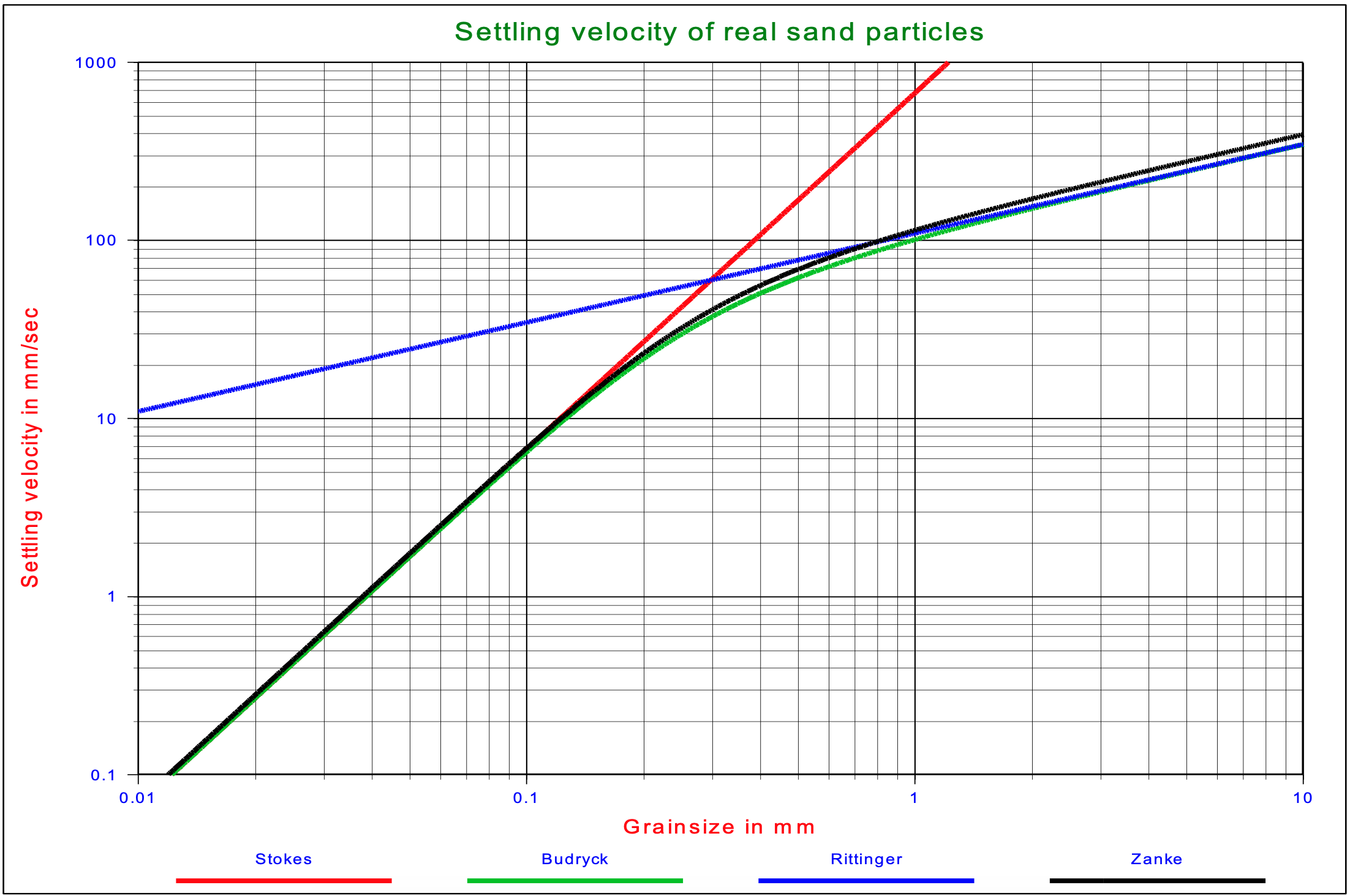
Figure 4.4-2 shows the settling velocity as a function of the particle diameter for the Stokes, Budryck, Rittinger & Zanke equations.

Since the equations were derived for sand grains, the shape factor for sand grains is used for determining the constants in the equations. The shape factor can be introduced into the equations for the drag coefficient by dividing the drag coefficient by a shape factor \(\ \psi\). For normal sands this shape factor has a value of 0.7.

The viscosity of the water is temperature dependent. If a temperature of 10^o is used as a reference, then the viscosity increases by 27% at 0^o and it decreases by 30% at 20^o centigrade. Since the viscosity influences the Reynolds number, the settling velocity for laminar settling is also influenced by the viscosity. For turbulent settling the drag coefficient does not depend on the Reynolds number, so this settling process is not influenced by the viscosity.

Other researchers use slightly different constants in these equations but, these equations suffice to explain the basics of the different slurry transport models.

Figure 4.4-1: The drag coefficient as a function of the particle Reynolds number.

Figure 4.4-2: The settling velocity of individual particles. The Huisman (1973-1995) Method.

The Huisman (1973-1995) Method

A better approximation and more workable equations for the drag coefficient C_D may be obtained by subdividing the transition region, for instance:

\[\ \mathrm{R} \mathrm{e}_{\mathrm{p}}<\mathrm{1} \quad \mathrm{C}_{\mathrm{D}}=\frac{\mathrm{2 4}}{\mathrm{R e}_{\mathrm{p}}^{\mathrm{1}}}\]

\[\ \mathrm{1}<\mathrm{R} \mathrm{e}_{\mathrm{p}}<\mathrm{5 0} \quad \mathrm{C}_{\mathrm{D}}=\frac{\mathrm{2 4}}{\mathrm{R e}_{\mathrm{p}}^{3 / 4}}\]

\[\ \mathrm{5 0 < R e _ { p } < 1 6 2 0} \quad \mathrm{C}_{\mathrm{D}}=\frac{4.7}{\mathrm{R e}_{\mathrm{p}}^{1 / 3}}\]

\[\ \mathrm{1 6 2 0}<\mathrm{R e}_{\mathrm{p}} \quad \mathrm{C}_{\mathrm{D}}=\mathrm{0 . 4}\]

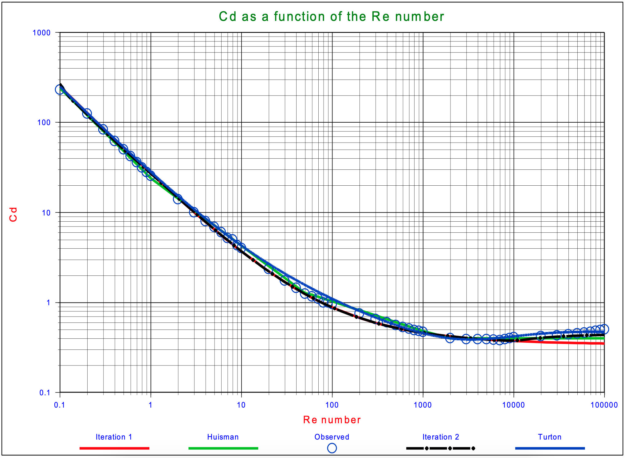
This power approximation is also shown in Figure 4.4-1. Substitution of these equations in equation (4.2-5) gives:

\[\ \mathrm{R} \mathrm{e}_{\mathrm{p}}<\mathrm{1} \quad \mathrm{v}_{\mathrm{t}}=\frac{\mathrm{1}}{\mathrm{1 8}} \cdot \frac{\mathrm{g}^{\mathrm{1}}}{v_{\mathrm{l}}^{\mathrm{1}}} \cdot \mathrm{R}_{\mathrm{s} \mathrm{d}}^{\mathrm{1}} \cdot \mathrm{d}^{\mathrm{2}}\]

\[\ \mathrm{1}<\mathrm{R} \mathrm{e}_{\mathrm{p}}<\mathrm{5 0} \quad \mathrm{v}_{\mathrm{t}}=\frac{\mathrm{1}}{\mathrm{1 0}} \cdot \frac{\mathrm{g}^{\mathrm{0 . 8}}}{v_{\mathrm{l}}^ {\mathrm{0 . 6}}} \cdot \mathrm{R}_{\mathrm{s d}}^{\mathrm{0 . 8}} \cdot \mathrm{d}^{\mathrm{1 . 4}}\]

\[\ \mathrm{5 0}<\mathrm{R e}_{\mathrm{p}}<\mathrm{1 6 2 0} \quad \mathrm{v}_{\mathrm{t}}=\frac{\mathrm{1}}{\mathrm{2 . 1 3}} \cdot \frac{\mathrm{g}^{\mathrm{0 . 6}}}{v_{\mathrm{l}}^ {\mathrm{0 . 2}}} \cdot \mathrm{R}_{\mathrm{s d}}^{\mathrm{0 . 6}} \cdot \mathrm{d}^{\mathrm{0 . 8}}\]

\[\ \mathrm{1 6 2 0}<\mathrm{R} \mathrm{e}_{\mathrm{p}} \quad \mathrm{v}_{\mathrm{t}}=1.83 \cdot \frac{\mathrm{g}^{\mathrm{0 . 5}}}{\mathrm{v}_{\mathrm{l}}^{\mathrm{0}}} \cdot \mathrm{R}_{\mathrm{s} \mathrm{d}}^{\mathrm{0 . 5}} \cdot \mathrm{d}^{\mathrm{0 . 5}}\]

These equations are difficult to use in an actual case because the value of Re_p depends on the terminal settling velocity. The following method gives a more workable solution.

Equation (4.2-5) can be transformed into:

\[\ \mathrm{C}_{\mathrm{D}} \cdot \mathrm{R} \mathrm{e}_{\mathrm{p}}^{\mathrm{2}}=\frac{\mathrm{4}}{\mathrm{3}} \cdot \mathrm{R}_{\mathrm{s} \mathrm{d}} \cdot \frac{\mathrm{g}}{v_{\mathrm{l}}^{\mathrm{2}}} \cdot \mathrm{d}^{\mathrm{3}}\]

This factor can be determined from the equations above:

\[\ \mathrm{R e}_{\mathrm{p}}<\mathrm{1} \quad \mathrm{C}_{\mathrm{D}} \cdot \mathrm{R} \mathrm{e}_{\mathrm{p}}^{\mathrm{2}}=\mathrm{2 4} \cdot \mathrm{R} \mathrm{e}_{\mathrm{p}}\]

\[\ \mathrm{1}<\mathrm{R} \mathrm{e}_{\mathrm{p}}<\mathrm{5 0} \quad \mathrm{C}_{\mathrm{D}} \cdot \mathrm{R} \mathrm{e}_{\mathrm{p}}^{2}=\mathrm{2 4} \cdot \mathrm{R} \mathrm{e}_{\mathrm{p}}^{\mathrm{5} / 4}\]

\[\ \mathrm{5 0}<\mathrm{R} \mathrm{e}_{\mathrm{p}}<\mathrm{1 6 2 0} \quad \mathrm{C}_{\mathrm{D}} \cdot \mathrm{R} \mathrm{e}_{\mathrm{p}}^{\mathrm{2}}=\mathrm{4 . 7} \cdot \mathrm{R} \mathrm{e}_{\mathrm{p}}^{\mathrm{5} / \mathrm{3}}\]

\[\ \mathrm{1 6 2 0}<\mathrm{R e}_{\mathrm{p}} \quad \mathrm{C}_{\mathrm{D}} \cdot \mathrm{R e}_{\mathrm{p}}^{2}=\mathrm{0 . 4} \cdot \mathrm{R e}_{\mathrm{p}}^{2}\]

From these equations the equation to be applied can be picked and the value of Re_p calculated. The settling velocity now follows from:

\[\ \mathrm{v}_{\mathrm{t}}=\mathrm{R} \mathrm{e}_{\mathrm{p}} \cdot \frac{v_{\mathrm{l}}}{\mathrm{d}}\]

The Grace Method (1986)

Following the suggestions of Grace (1986), it is found convenient to define a dimensionless particle diameter, which in fact is the Bonneville parameter (d in m and v_t in m/s):

\[\ \mathrm{D}_{*}=\mathrm{d} \cdot\left(\frac{\mathrm{R}_{\mathrm{sd}} \cdot \mathrm{g}}{v_{\mathrm{l}}^{2}}\right)^{\mathrm{1} / 3}\]

And a dimensionless terminal settling velocity:

\[\ \mathrm{v}_{\mathrm{t}}^{*}=\mathrm{v}_{\mathrm{t}} \cdot\left(\frac{\mathrm{1}}{v_{\mathrm{l}} \cdot \mathrm{R}_{\mathrm{s} \mathrm{d}} \cdot \mathrm{g}}\right)^{\mathrm{1} / \mathrm{3}}\]

Those are mutually related. Thus using the curve and rearranging gives directly the velocity v_t as a function of particle diameter d. No iteration is required. This described by analytic expressions appropriate for a computational determination of v_t according to Grace Method. Now v_t can be computed according to:

\[\ \mathrm{v}_{\mathrm{t}}=\mathrm{v}_{\mathrm{t}}^{*} \cdot\left(\frac{\mathrm{1}}{v_{\mathrm{l}} \cdot \mathrm{R}_{\mathrm{s} \mathrm{d}} \cdot \mathrm{g}}\right)^{-\mathrm{1} / \mathrm{3}}\]

\[\ \mathrm{D}^{*}<\mathrm{3 . 8} \quad\quad \mathrm{v}_{\mathrm{t}}^{*}=\frac{\left(\mathrm{D}^{*}\right)^{2}}{\mathrm{1 8}}-\mathrm{3 . 1 2 3 4} \cdot \mathrm{1 0}^{-4} \cdot\left(\mathrm{D}^{*}\right)^{5}+\mathrm{1 . 6 4 1 5} \cdot \mathrm{1 0}^{-\mathrm{6}} \cdot\left(\mathrm{D}^{*}\right)^{\mathrm{8}} -7.27 \mathrm{8} \cdot \mathrm{1 0}^{-10} \cdot\left(\mathrm{D}^{*}\right)^{11}\]

\[\ 3.8<\mathrm{D}^{*}<7.58 \quad \mathrm{v}_{\mathrm{t}}^{*}=\mathrm{1 0}^{-\mathrm{1 . 5 4 4 6}+2.9162 \cdot \log \left(\mathrm{D}^{*}\right)-\mathrm{1 . 0 4 3 2} \cdot \log \left(\mathrm{D}^{*}\right)^{2}}\]

\[\ 7.58<D^{*}<227 \quad \mathrm{v_{t}^{*}}=10^{-1.64758+2.94786 \cdot \log \left(D^{*}\right)-1.09703 \cdot \log \left(D^{*}\right)^{2}+0.17129 \cdot \log \left(D^{*}\right)^{3}}
\]

\[\ 227<D^{*}<3500 \quad \mathrm{v_{t}^{*}}=10^{5.1837-4.51034 \cdot \log \left(D^{*}\right)+1.687 \cdot \log \left(D^{*}\right)^{2}-0.189135 \cdot \log \left(D^{*}\right)^{3}}\]

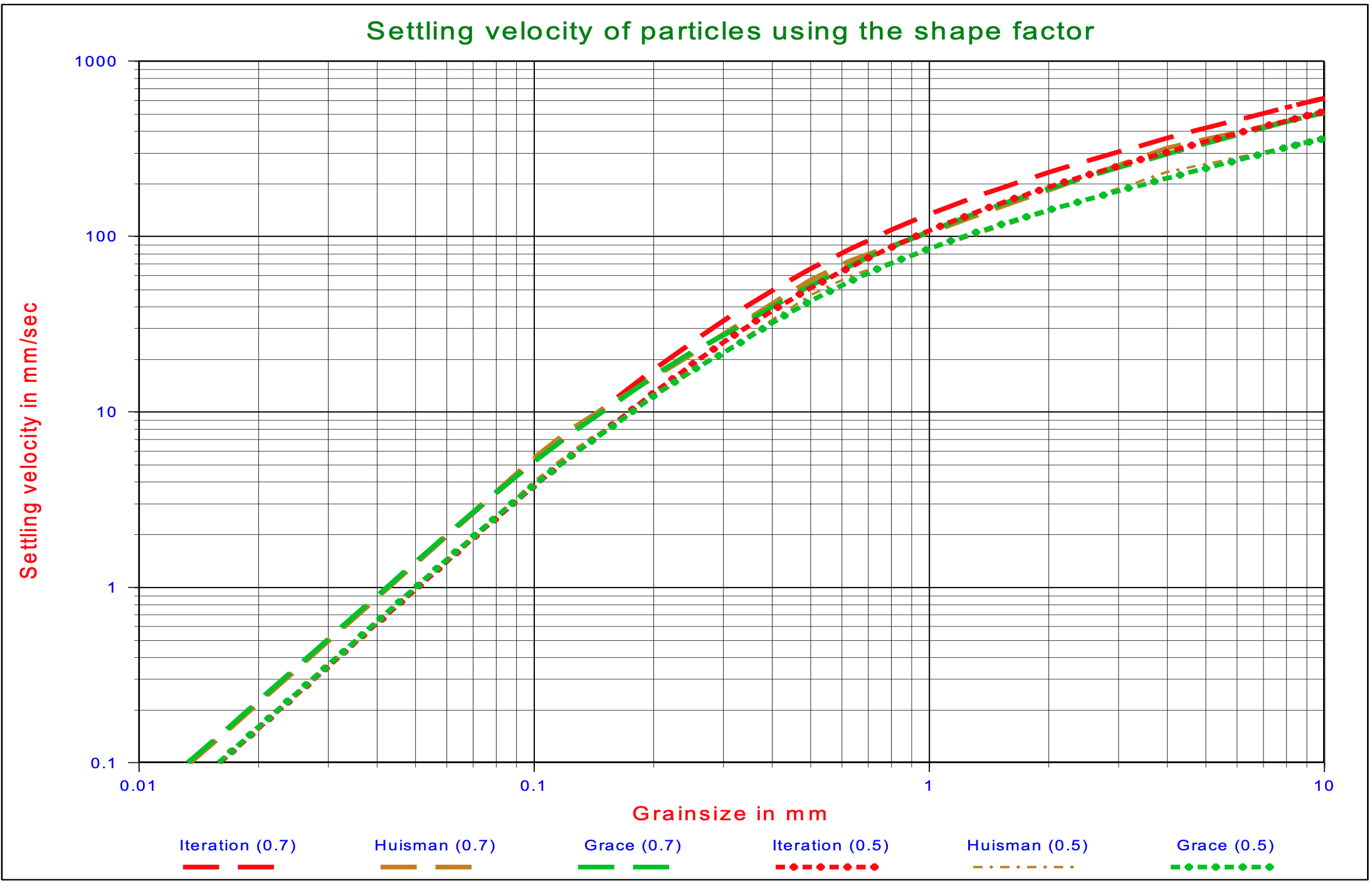
Figure 4.4-3 shows the terminal settling velocity for the iterative method according to equations (4.3-4), (4.3-5) and (4.3-6) and the methods of Huisman (1973-1995) and Grace (1986), using shape factors of 0.5 and 0.7. It can be seen that for small diameters these methods gives smaller velocities while for larger diameters larger velocities are predicted, compared with the other equations as shown in Figure 4.4-2. The iterative method gives larger velocities for the larger diameters, compared with the Huisman and Grace methods, but this is caused by the different way of implementing the shape factor. In the iterative method the shape factor is implemented according to equation 2, while with the Huisman and Grace methods the terminal settling velocity for spheres is multiplied by the shape factor according to equation (4.5-1). For the smaller grain diameters, smaller than 0.5 mm, which are of interest here, the 3 methods give the same results.

Figure 4.4-3: The settling velocity of individual particles using the shape factor.