6.6: Silin, Kobernik and Asaulenko (1958) and (1962)

Last updated
Save as PDF

Page ID: 29225

\( \newcommand{\vecs}[1]{\overset { \scriptstyle \rightharpoonup} {\mathbf{#1}} } \) \( \newcommand{\vecd}[1]{\overset{-\!-\!\rightharpoonup}{\vphantom{a}\smash {#1}}} \)\(\newcommand{\id}{\mathrm{id}}\) \( \newcommand{\Span}{\mathrm{span}}\) \( \newcommand{\kernel}{\mathrm{null}\,}\) \( \newcommand{\range}{\mathrm{range}\,}\) \( \newcommand{\RealPart}{\mathrm{Re}}\) \( \newcommand{\ImaginaryPart}{\mathrm{Im}}\) \( \newcommand{\Argument}{\mathrm{Arg}}\) \( \newcommand{\norm}[1]{\| #1 \|}\) \( \newcommand{\inner}[2]{\langle #1, #2 \rangle}\) \( \newcommand{\Span}{\mathrm{span}}\) \(\newcommand{\id}{\mathrm{id}}\) \( \newcommand{\Span}{\mathrm{span}}\) \( \newcommand{\kernel}{\mathrm{null}\,}\) \( \newcommand{\range}{\mathrm{range}\,}\) \( \newcommand{\RealPart}{\mathrm{Re}}\) \( \newcommand{\ImaginaryPart}{\mathrm{Im}}\) \( \newcommand{\Argument}{\mathrm{Arg}}\) \( \newcommand{\norm}[1]{\| #1 \|}\) \( \newcommand{\inner}[2]{\langle #1, #2 \rangle}\) \( \newcommand{\Span}{\mathrm{span}}\)\(\newcommand{\AA}{\unicode[.8,0]{x212B}}\)

Silin, Kobernik & Asaulenko (1958) & (1962) carried out experiment in pipes with diameters of 0.024 m, 0.103 m, 0.206 m, 0.308 m, 0.410 m, 0.614 m, 0.800 m and 0.900 m. They used particles with diameters of 0.16 mm, 0.23 mm, 0.25 mm, 0.29 mm, 0.33 mm, 0.41 mm, 0.65 mm, 1 mm and 2 mm. The relative submerged densities used were 0.59, 0.85, 1.59 and 2.28. Most probably they used more pipe diameters, particle diameters and relative submerged densities, since most of the original reports are in Russian and difficult to find. The experiments are however very valuable, since a broad range of pipe diameters is covered.

Figure 6.6-1 shows the Durand Froude F_L numbers found for pipe diameters of 0.1 m, 0.2 m and 0.3 m. The graph also shows the Jufin & Lopatin F_L curve and the DHLLDV F_L curve. If only sand particles are considered, it looks like the F_L value decreases slightly with the pipe diameter. This is also part of the Jufin & Lopatin (1966) equation for the LDV, which is based on these experiments. If also other relative submerged densities are considered, it looks like the F_L value increases with decreasing relative submerged density. One should however also consider the volumetric concentrations that may influence the F_L values. The Jufin & Lopatin (1966) curve in the graph is for an 0.3 m pipe, for the smaller pipe diameters the curve is slightly higher.

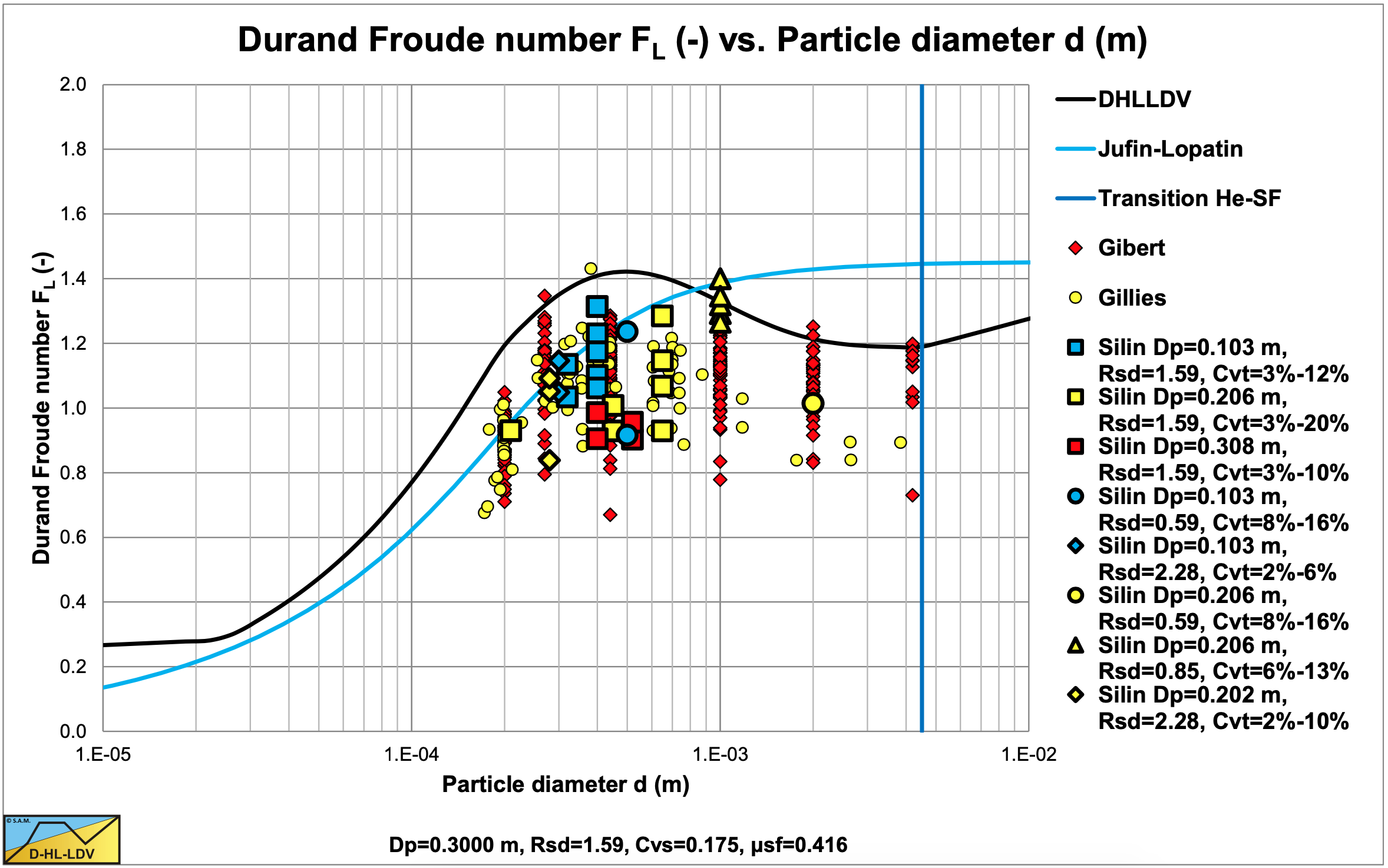
Screen Shot 2020-07-14 at 10.27.02 AM.png

Figure 6.6-2, Figure 6.6-3, Figure 6.6-4, Figure 6.6-5, Figure 6.6-6 and Figure 6.6-7 show results of experiments carried out by Silin et al. (1958) and used by Jufin & Lopatin (1966) for their model. Figure 6.6-2, Figure 6.6-4 and Figure 6.6-6 show the original data in i_m vs. v_ls graphs, while Figure 6.6-3, Figure 6.6-5, and Figure 6.6-7 show processed data in E_rhg vs. i_l graphs. These experiments are very valuable, since they were carried out in large diameter pipes. The experiments show a lot of scatter, especially in the E_rhg vs. i_lgraphs. A general conclusion of these experiments is, that the hydraulic gradient is best estimated with the ELM model.

The Jufin & Lopatin (1966) model, based on these experiments, assumes that the excess head losses are proportional to the square root of the concentration and not linear with the concentration. Analyzing the data shows that part of the data points is in the heterogeneous flow regime and part is in the (pseudo) homogeneous flow regime. For the homogeneous flow regime other researchers have already observed that the excess hydraulic gradient is between 0 and the excess hydraulic gradient of the ELM. This would match the Jufin & Lopatin (1966) observations. Whether this is also true in the heterogeneous flow regime is however contradictory with the observations of most other researchers. Mixing two flow regimes into 1 equation/model is not a good idea, since the physics of both flow regimes differ.

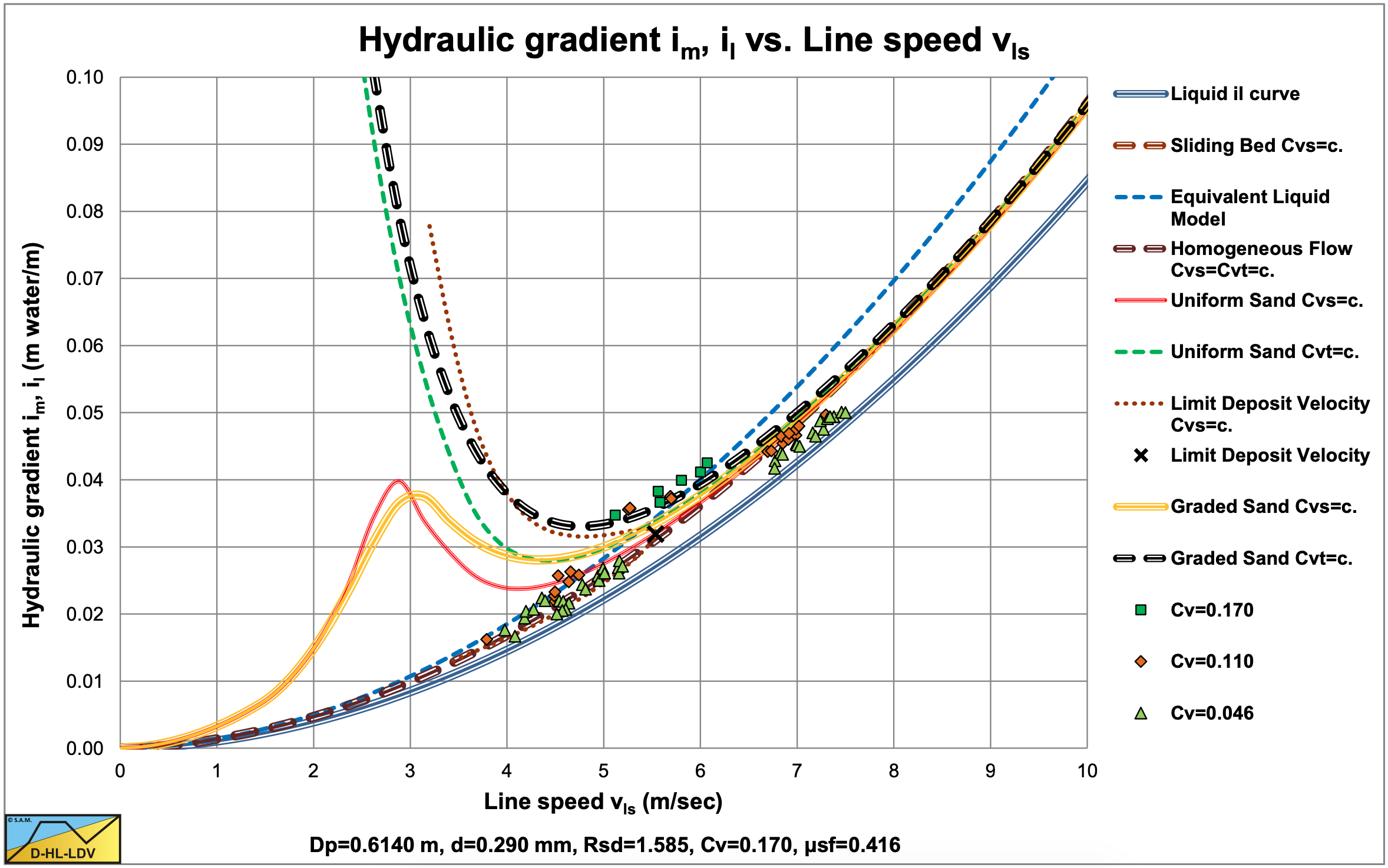
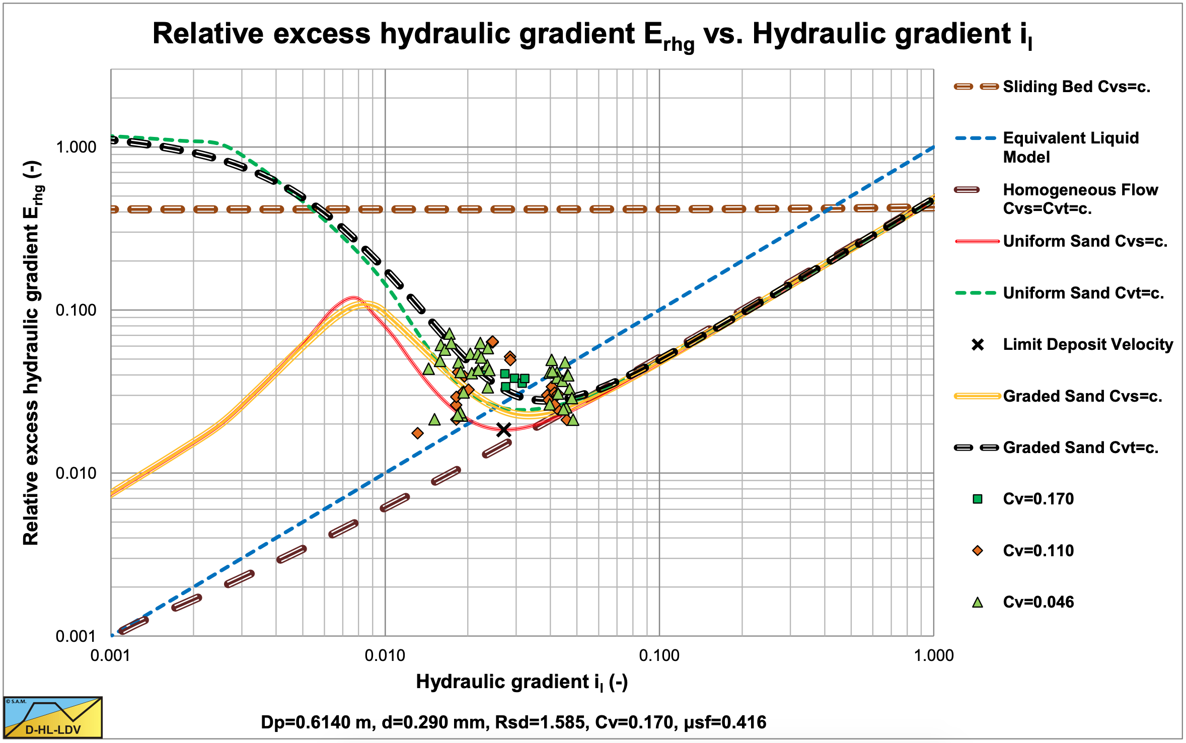
Screen Shot 2020-07-14 at 10.30.12 AM.png

Screen Shot 2020-07-14 at 10.31.18 AM.png

Figure 6.6-2 and Figure 6.6-3 show the data versus the DHLLDV Framework for uniform and graded sands (more realistic). The data points match the graded curve reasonably. Figure 6.6-2 is for a concentration of 17%. These data points match. Figure 6.6-3 is almost dimensionless and shows the match of all data points. The data points can be divided into two groups. The group on the left is in the heterogeneous flow regime, while the group on the right is more at the transition of the heterogeneous flow regime to the homogeneous flow regime.

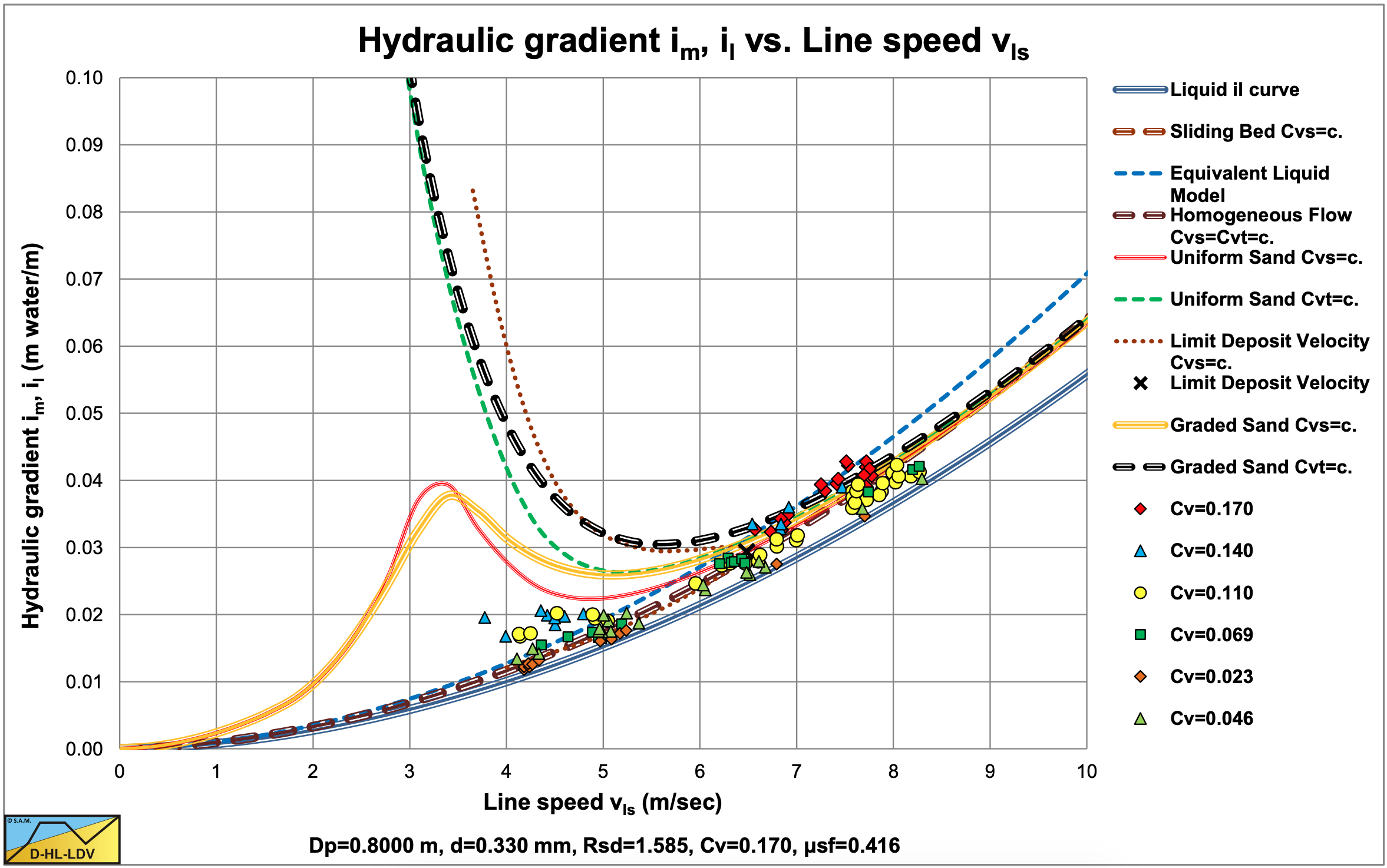
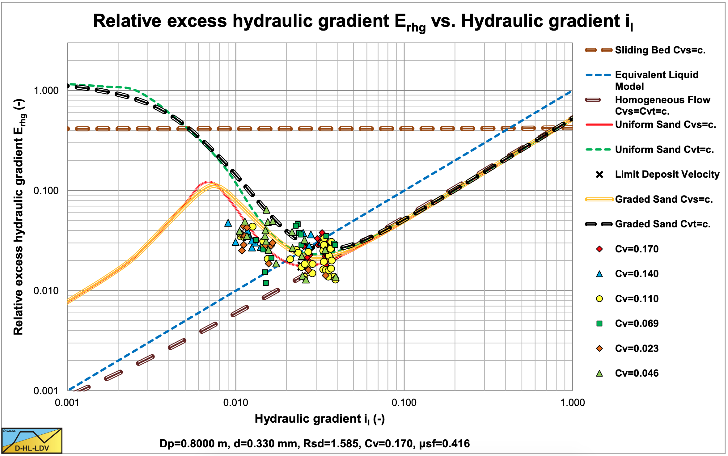
Screen Shot 2020-07-14 at 10.37.55 AM.png

Screen Shot 2020-07-14 at 10.38.55 AM.png

Figure 6.6-4 and Figure 6.6-5 show the data versus the DHLLDV Framework for uniform and graded sands (more realistic). The data points match the graded curve reasonably. Figure 6.6-4 is for a concentration of 17%. These data points match. Figure 6.6-5 is almost dimensionless and shows the match of all data points. The data points can be divided into two groups. The group on the left is in the heterogeneous flow regime, while the group on the right is more at the transition of the heterogeneous flow regime to the homogeneous flow regime.

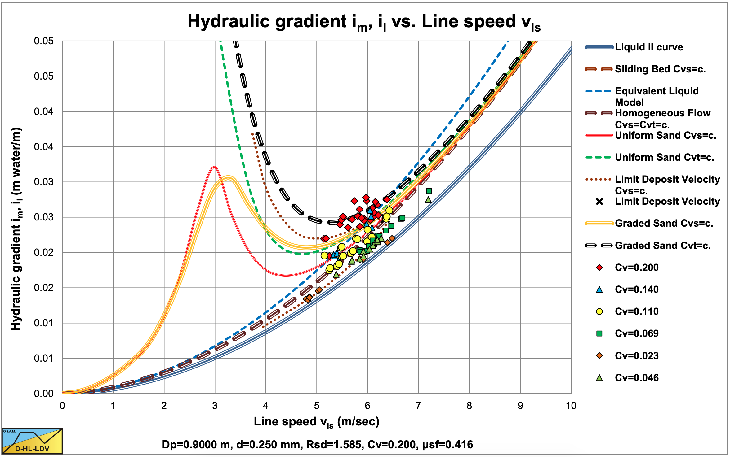
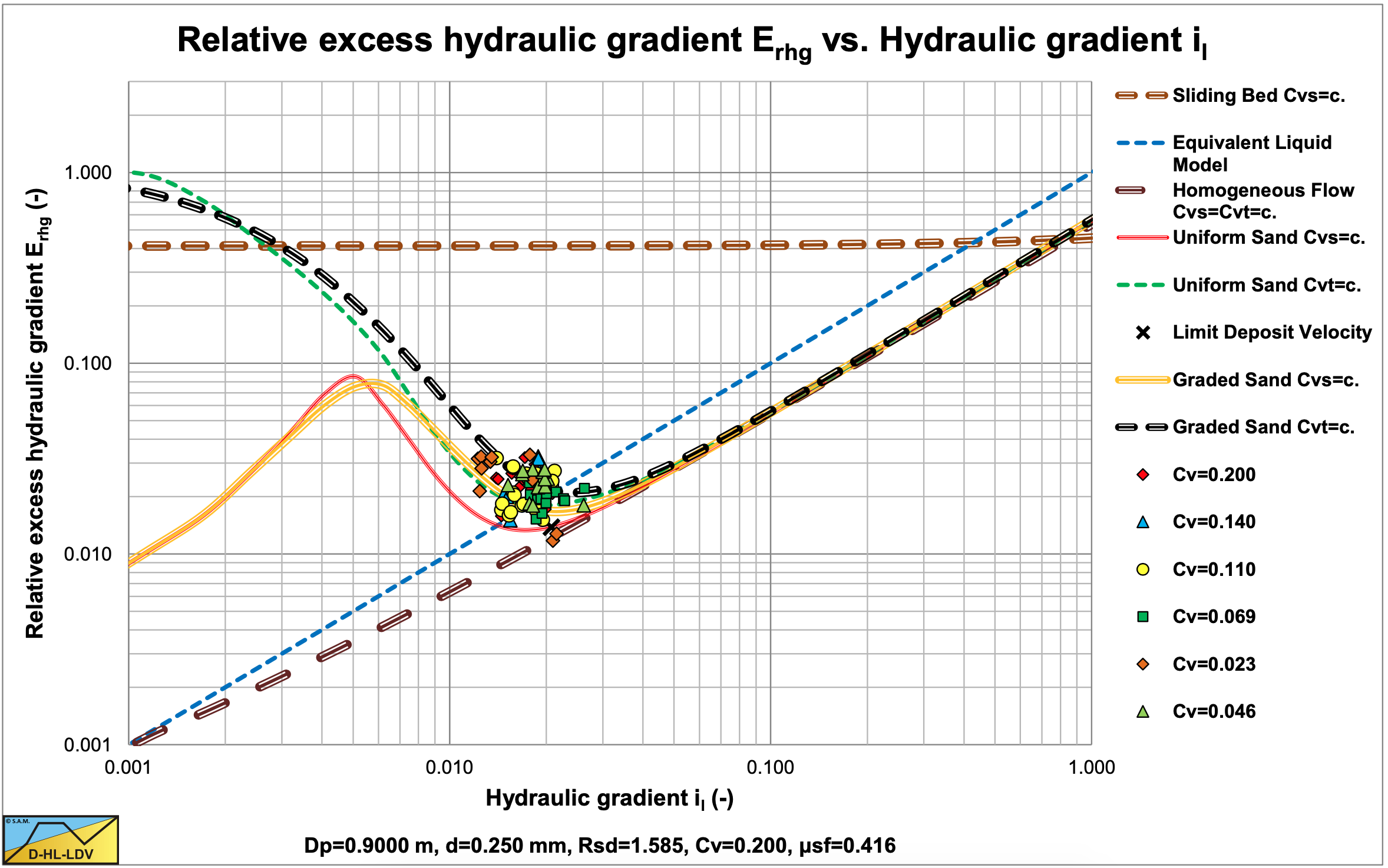
Screen Shot 2020-07-14 at 10.40.28 AM.png

Screen Shot 2020-07-14 at 10.41.22 AM.png

Figure 6.6-6 and Figure 6.6-7 show the data versus the DHLLDV Framework for uniform and graded sands (more realistic). The data points match the graded curve reasonably. Figure 6.6-6 is for a concentration of 20%. These data points match. Figure 6.6-5 is almost dimensionless and shows the match of all data points. The data points can be divided into two groups. The group on the left is in the heterogeneous flow regime, while the group on the right is more at the transition of the heterogeneous flow regime to the homogeneous flow regime.