6.13: Conclusions and Discussion Empirical and Semi-Empirical Models

6.16.1 Introduction

About 60 years after Durand & Condolios (1952) and Newitt et al. (1955) carried out their research, their results are still valid and important. In spite of criticism of Zandi & Govatos (1967), Babcock (Babcock, 1970), Wilson et al. (1992) and others, their equations are still widely used. There are some issues identified, leading to a wrong interpretation of the equations. The main issues are; the wrong use of the particle Froude number √C_x vs. the drag coefficient C_D, the wrong use of the relative submerged density R_sd in the particle Froude number √C_x, the wrong power of the particle Froude number √C_x and the use of the wrong graph for the Limit Deposit Velocity coefficient F_L in the Durand & Condolios (1952) equations. For the Limit Deposit Velocity coefficient F_L the correction factor of about 1.1 according to Gibert (1960) should be applied. For Newitt et al. (1955) it should be considered that the sliding bed equation is based on an average of some specific materials in a very small pipe (1 inch). Other materials and pipes may lead to sliding friction coefficients in the range of μ_sf=0.35-0.7. Combining both theories results in a flow regime chart as is shown in Figure 6.5-4 and Figure 6.5-5. In these charts the Newitt et al. (1955) equations are used for the transition moving bed-heterogeneous transport and heterogeneous-homogeneous transport. The Durand & Condolios (1952) approach is used for the stationary bed curve.

Both Durand & Condolios (1952) and Newitt et al. (1955) consider the excess pressure losses for heterogeneous transport to be reversely proportional to the line speed. Zandi & Govatos (1967) found a power of -1.93 and Wilson et al. (1992) a power of -1.7 for uniform particle size distributions and smaller powers up to -0.25 for non-uniform distributions. This leads to relative excess pressure powers of 3, 3.93 and 3.7. Now heterogeneous transport is dominated by the energy losses due to collisions of particles. If we assume that the occurrence of collisions is dominated by the settling velocity of the particles, then the number of collisions per unit of time is almost independent of time and thus of the line speed. This implies that the number of collisions per unit of pipeline length is reversely proportional to the line speed, resulting in a power of -1 of the line speed in the excess pressure losses or -3 in the relative excess pressure losses. If one considers the momentum of the particles in the direction of the line speed, higher powers can be explained.

The final conclusion is, that the 60 year old theories can still be applied if one takes the effort to use them properly.

6.16.2 The Darcy-Weisbach Friction Factor

The Darcy-Weisbach friction factor of a smooth pipe in a dimensionless form can be determined by:

\[\ \mathrm{\lambda_{l}=0.01216 \cdot\left(v_{l s}\right)^{-0.155} \cdot\left(D_{p}\right)^{-0.175} \approx 0.1233 \cdot\left(v_{l s}\right)^{-0.155} \cdot\left(g \cdot D_{p}\right)^{-0.172} \cdot\left(v_{l} \cdot g\right)^{1 / 6}}\]

This equation will be substituted in the hydraulic gradient equations in order to get expressions based on the parameters users (dredging companies) know. These are the pipe diameter D_p, the cross section averaged line speed v_ls and some characteristic particle diameter d or maybe the PSD. Normally in dredging the solids will be sand or gravel consisting of quarts with a relative submerged density R_sd of 1.58-1.65 ton/m³ (depending on the water density, 1.000-1.030 ton/m³). The kinematic viscosity of water depends on the temperature, at 10°C ν=0.0000013 m²/sec, at 20°C ν=0.0000010 m²/sec.

6.16.3 Heterogeneous Regime

In order to compare a number of models, the models have to be written in the same form. To do so the form of Fuhrboter (1961) is chosen, the hydraulic gradient of a mixture consists of the liquid hydraulic gradient plus the solids effect. With the solids effect factor S_k (to compare with Fuhrboter) defined as:

\[\ \mathrm{i}_{\mathrm{m}}=\mathrm{i}_{\mathrm{l}}+\mathrm{S}_{\mathrm{k}} \cdot \frac{\mathrm{C}_{\mathrm{v} \mathrm{t}}}{\mathrm{v}_{\mathrm{ls}}}\]

The models chosen for this comparison all have a solids effect reversely proportional to the cross section averaged line speed.

6.16.3.1 Durand & Condolios (1952)

The hydraulic gradient of a mixture according to Durand & Condolios (1952) is:

\[\ \begin{array}{left} \mathrm{i}_{\mathrm{m}} &=\mathrm{i}_{\mathrm{l}}+\mathrm{8 5} \cdot\left(\frac{\mathrm{v}_{\mathrm{l} \mathrm{s}}^{\mathrm{2}} \cdot \mathrm{C}_{\mathrm{x}}^{\mathrm{1 0} / \mathrm{9}}}{\mathrm{g} \cdot \mathrm{D}_{\mathrm{p}} \cdot \mathrm{R}_{\mathrm{s d}}}\right)^{-\mathrm{3} / \mathrm{2}} \cdot \mathrm{C}_{\mathrm{v t}} \cdot \frac{\lambda_{\mathrm{l}} \cdot \mathrm{v}_{\mathrm{l} \mathrm{s}}^{2}}{\mathrm{2} \cdot \mathrm{g} \cdot \mathrm{D}_{\mathrm{p}}} \\ &=\mathrm{i}_{\mathrm{l}}+\mathrm{4} \mathrm{2 . 5} \cdot \lambda_{\mathrm{l}} \cdot\left(\mathrm{g} \cdot \mathrm{D}_{\mathrm{p}}\right)^{\mathrm{1 / 2}} \cdot\left(\frac{\mathrm{R}_{\mathrm{s d}}}{\mathrm{C}_{\mathrm{x}}^{\mathrm{1 0} / \mathrm{9}}}\right)^{\mathrm{3} / 2} \cdot \frac{\mathrm{C}_{\mathrm{v} \mathrm{t}}}{\mathrm{v}_{\mathrm{ls}}} \end{array}\]

The hydraulic gradient can be determined by, after substituting of the Darcy-Weisbach friction factor:

\[\ \mathrm{i}_{\mathrm{m}}=\mathrm{i}_{\mathrm{l}}+\mathrm{5} . \mathrm{2 4} \cdot\left(v_{\mathrm{l}} \cdot \mathrm{g}\right)^{\mathrm{1} / \mathrm{6}} \cdot\left(\mathrm{g} \cdot \mathrm{D}_{\mathrm{p}}\right)^{\mathrm{0 . 3 2 8}} \cdot\left(\frac{\mathrm{R}_{\mathrm{s d}}}{\mathrm{C}_{\mathrm{x}}^{\mathrm{1 0} / 9}}\right)^{\mathrm{3} / 2} \cdot \frac{\mathrm{1}}{\mathrm{v}_{\mathrm{l} \mathrm{s}}^{\mathrm{0 . 1 5 5}}} \cdot \frac{\mathrm{C}_{\mathrm{v t}}}{\mathrm{v}_{\mathrm{l s}}}\]

This gives for the solids effect factor S_k:

\[\ \mathrm{S_{k}=5.24}{ \cdot\left(v_{\mathrm{l}} \cdot \mathrm{g}\right)^{1 / 6} \mathrm{\cdot\left(g \cdot D_{p}\right)^{0.328} \cdot\left(\frac{R_{s d}}{C_{x}^{10 / 9}}\right)^{3 / 2} \cdot \frac{1}{v_{l s}^{0.155}}}}\]

6.16.3.2 Newitt et al. (1955)

The hydraulic gradient of a mixture according to Newitt et al. (1955) is:

\[\ \begin{array}{left} \mathrm{i}_{\mathrm{m}} &=\mathrm{i}_{\mathrm{l}}+\mathrm{1 1 0 0} \cdot\left(\mathrm{g} \cdot \mathrm{D}_{\mathrm{p}} \cdot \mathrm{R}_{\mathrm{s d}}\right) \cdot \mathrm{v}_{\mathrm{t}} \cdot \mathrm{C}_{\mathrm{v t}} \cdot\left(\frac{\mathrm{1}}{\mathrm{v}_{\mathrm{l s}}}\right)^{3} \cdot \frac{\lambda_{\mathrm{l}} \cdot \mathrm{v}_{\mathrm{l s}}^{2}}{\mathrm{2} \cdot \mathrm{g} \cdot \mathrm{D}_{\mathrm{p}}} \\ &=\mathrm{i}_{\mathrm{l}}+\mathrm{5 5 0} \cdot \lambda_{\mathrm{l}} \cdot \mathrm{R}_{\mathrm{s d}} \cdot \mathrm{v}_{\mathrm{t}} \cdot \frac{\mathrm{C}_{\mathrm{v} \mathrm{t}}}{\mathrm{v}_{\mathrm{ls}}} \end{array}\]

The hydraulic gradient can be determined by, after substituting of the Darcy-Weisbach friction factor:

\[\ \mathrm{i}_{\mathrm{m}}=\mathrm{i}_{\mathrm{l}}+\mathrm{67.8} \cdot \frac{\left(v_{\mathrm{l}} \cdot \mathrm{g}\right)^{1 / 6} \cdot \mathrm{R}_{\mathrm{s d}} \cdot \mathrm{v}_{\mathrm{t}}}{\left(\mathrm{g} \cdot \mathrm{D}_{\mathrm{p}}\right)^{0.172}} \cdot \frac{\mathrm{1}}{\mathrm{v}_{\mathrm{l} \mathrm{s}}^{0.155}} \cdot \frac{\mathrm{C}_{\mathrm{v} \mathrm{t}}}{\mathrm{v}_{\mathrm{l s}}}\]

This gives for the solids effect factor S_k:

\[\ \mathrm{ S_{k}}=67.8 \cdot \frac{\left(v_{1} \cdot \mathrm{g}\right)^{1 / 6} \cdot \mathrm{R_{s d} \cdot v_{t}}}{\left(\mathrm{g \cdot D_{p}}\right)^{0.172}} \cdot \frac{1}{\mathrm{v_{l s}^{0.155}}}\]

6.16.3.3 Fuhrboter (1961)

Fuhrboter (1961) already used the notation with solids effect and gave the S_k value in a graph.

\[\ \mathrm{i}_{\mathrm{m}}=\mathrm{i}_{\mathrm{l}}+\mathrm{S}_{\mathrm{k}} \cdot \frac{\mathrm{C}_{\mathrm{v} \mathrm{t}}}{\mathrm{v}_{\mathrm{ls}}}\]

Now Fuhrboter (1961) assumed the S_k value was proportional with the particle diameter for medium sands and also assumed the terminal setting velocity v_t=100·d. This way the S_k value is proportional to the terminal setting velocity v_t.

6.16.3.4 Jufin & Lopatin (1966) Group B

The hydraulic gradient of a mixture according to Jufin & Lopatin (1966) is:

\[\ \begin{array}{left}\mathrm{i}_{\mathrm{m}}&=\mathrm{i}_{1}+2 \cdot 90389 \cdot\left(\mathrm{g} \cdot \mathrm{D}_{\mathrm{p}} \cdot \mathrm{R}_{\mathrm{sd}} \cdot \Psi^{*}\right)^{1 / 2} \cdot\left(v_{1} \cdot \mathrm{g}\right)^{2 / 3} \cdot\left(\mathrm{C}_{\mathrm{vt}}\right)^{1 / 2}\left(\frac{1}{\mathrm{v}_{\mathrm{ls}}}\right)^{3} \cdot \frac{\lambda_{\mathrm{l}} \cdot \mathrm{v}_{\mathrm{ls}}^{2}}{2 \cdot \mathrm{g} \cdot \mathrm{D}_{\mathrm{p}}}\\
&=\mathrm{i}_{\mathrm{l}}+90389 \cdot \frac{\lambda_{\mathrm{l}} \cdot\left(\Psi^{*} \cdot \mathrm{R}_{\mathrm{sd}}\right)^{1 / 2} \cdot\left(v_{\mathrm{l}} \cdot \mathrm{g}\right)^{2 / 3}}{\left(\mathrm{g} \cdot \mathrm{D}_{\mathrm{p}}\right)^{1 / 2} \cdot\left(\mathrm{C}_{\mathrm{vt}}\right)^{1 / 2}} \cdot \frac{\mathrm{C}_{\mathrm{vt}}}{\mathrm{v}_{\mathrm{ls}}}\end{array}\]

The hydraulic gradient can be determined by, after substituting of the Darcy-Weisbach friction factor:

\[\ \mathrm{i}_{\mathrm{m}}=\mathrm{i}_{\mathrm{l}}+\mathrm{1 1 1 4 5} \cdot \frac{\left(\Psi^{*} \cdot \mathrm{R}_{\mathrm{s d}}\right)^{1 / 2} \cdot\left(v_{\mathrm{l}} \cdot \mathrm{g}\right)^{\mathrm{5} / \mathrm{6}}}{\left(\mathrm{g} \cdot \mathrm{D}_{\mathrm{p}}\right)^{0.672} \cdot\left(\mathrm{C}_{\mathrm{v t}}\right)^{1 / 2}} \cdot \frac{\mathrm{1}}{\mathrm{v}_{\mathrm{l s}}^{\mathrm{0 . 1 5 5}}} \cdot \frac{\mathrm{C}_{\mathrm{v} \mathrm{t}}}{\mathrm{v}_{\mathrm{l s}}}\]

This gives for the solids effect factor S_k:

\[\ \mathrm{S_{k}=11145} \cdot \frac{\left(\Psi^{*} \cdot \mathrm{R_{s d}}\right)^{1 / 2} \cdot\left(v_{\mathrm{l}} \cdot \mathrm{g}\right)^{5 / 6}}{\left(\mathrm{g} \cdot \mathrm{D_{p}}\right)^{0.672} \cdot\left(\mathrm{C_{v t}}\right)^{1 / 2}} \cdot \frac{1}{\mathrm{v_{l s}}^{0.155}}\]

6.16.3.5 Wilson et al. (1992) Heterogeneous.

The hydraulic gradient of a mixture according to Wilson et al. (1992) is:

\[\ \mathrm{i}_{\mathrm{m}}=\mathrm{i}_{\mathrm{l}}+\frac{\mu_{\mathrm{s f}}}{2} \cdot \mathrm{C}_{\mathrm{v t}} \cdot \mathrm{R}_{\mathrm{s d}} \cdot\left(\frac{\mathrm{v}_{\mathrm{5} 0}}{\mathrm{v}_{\mathrm{l s}}}\right)=\mathrm{i}_{\mathrm{l}}+\frac{\mu_{\mathrm{s f}}}{2} \cdot \mathrm{R}_{\mathrm{s d}} \cdot \mathrm{v}_{\mathrm{5 0}} \cdot \frac{\mathrm{C}_{\mathrm{v} \mathrm{t}}}{\mathrm{v}_{\mathrm{l s}}}\]

This gives for the solids effect factor S_k:

\[\ \mathrm{S_{k}=\frac{\mu_{s f}}{2} \cdot R_{s d} \cdot v_{50}}\]

For the line speed, where 50% of the particles is in granular contact, v50, Wilson et al. (1992) give the following equation:

\[\ \mathrm{v}_{50}=\mathrm{w}_{50} \cdot \sqrt{\frac{\mathrm{8}}{\lambda_{\mathrm{l}}}} \cdot \cosh \left(\frac{\mathrm{6 0} \cdot \mathrm{d}_{50}}{\mathrm{D}_{\mathrm{p}}}\right)\]

The terminal settling velocity related parameter w, the particle associated velocity, can be determined by:

\[\ \mathrm{w}=\mathrm{0 . 9} \cdot \mathrm{v}_{\mathrm{t}}+\mathrm{2 . 7} \cdot\left(\mathrm{R}_{\mathrm{s d}} \cdot \mathrm{g} \cdot v_{\mathrm{l}}\right)^{1 / 3}\]

The terminal settling velocity v_t (strong), the pipe diameter D_p (weak), the particle diameter d₅₀ (weak), the line speed v_ls (weak) and the kinematic viscosity ν_l (weak) are all present in the characteristic velocity v₅₀. The model of Wilson can be simplified with some fit functions, according to:

\[\ \mathrm{v}_{\mathrm{5 0}} \approx \mathrm{3 . 9 3} \cdot\left(\mathrm{1 0 0 0} \cdot \mathrm{d}_{\mathrm{5 0}}\right)^{\mathrm{0 . 3 5}} \cdot\left(\frac{\mathrm{R}_{\mathrm{s d}}}{\mathrm{1 . 6 5}}\right)^{\mathrm{0 . 4 5}} \cdot\left(\frac{v_{\mathrm{l}, \mathrm{a c t u a l}}}{\mathrm{v}_{\mathrm{w}, \mathrm{2 0}}}\right)^{\mathrm{0 . 2 5}}\]

This gives for the S_k factor:

\[\ \mathrm{S}_{\mathrm{k}}=\mathrm{5 5 5} \cdot \mu_{\mathrm{s f}} \cdot \mathrm{d}_{\mathrm{5 0}}^{\mathrm{0.35}} \cdot \mathrm{R}_{\mathrm{s d}}^{\mathrm{1 . 4 5}} \cdot {v _ { \mathrm{l} }}^{\mathrm{0 . 2 5}}\]

6.16.3.6 DHLLDV Graded, Miedema (2014)

The hydraulic gradient of a mixture according to Miedema (2014) is for graded sands and gravels is:

\[\ \mathrm{i}_{\mathrm{m}}=\mathrm{i}_{\mathrm{l}}+\left(\frac{\mathrm{v}_{\mathrm{t}} \cdot\left(\mathrm{1}-\frac{\mathrm{\mathrm{C}}_{\mathrm{v s}}}{\mathrm{\kappa}}\right)^{\beta}}{\mathrm{v}_{\mathrm{l} \mathrm{s}}}+\mathrm{1} . \mathrm{8 4 5}^{2} \cdot\left(\frac{\mathrm{1}}{\sqrt{\lambda_{\mathrm{l}}}}\right) \cdot\left(\frac{\mathrm{v}_{\mathrm{t}}}{\sqrt{\mathrm{g} \cdot \mathrm{d}}}\right)^{10 / 3} \cdot\left(\frac{\left(v_{\mathrm{l}} \cdot \mathrm{g}\right)^{1 / 3}}{\mathrm{v}_{\mathrm{l s}}}\right)^{1}\right) \cdot \mathrm{R}_{\mathrm{sd}} \cdot \mathrm{C}_{\mathrm{v} \mathrm{s}}\]

Since the potential energy term (first term between brackets) is small compared to the kinetic energy term (second term between brackets) this can be simplified to:

\[\ \mathrm{i}_{\mathrm{m}}=\mathrm{i}_{\mathrm{l}}+\mathrm{1 . 8 4 5}^{2} \cdot\left(\frac{\mathrm{1}}{\lambda_{\mathrm{l}}}\right)^{1 / 2} \cdot\left(\frac{\mathrm{v}_{\mathrm{t}}}{\sqrt{\mathrm{g} \cdot \mathrm{d}}}\right)^{10 / 3} \cdot\left(v_{\mathrm{l}} \cdot \mathrm{g}\right)^{1 / 3} \cdot \mathrm{R}_{\mathrm{sd}} \cdot \frac{\mathrm{C}_{\mathrm{v} \mathrm{s}}}{\mathrm{v}_{\mathrm{l s}}}\]

The hydraulic gradient can be determined by, after substituting of the Darcy-Weisbach friction factor:

\[\ \mathrm{i}_{\mathrm{m}}=\mathrm{i}_{\mathrm{l}}+\mathrm{9 . 6 9} \cdot\left(\mathrm{g} \cdot \mathrm{D}_{\mathrm{p}}\right)^{0.086} \cdot\left(\frac{\mathrm{v}_{\mathrm{t}}}{\sqrt{\mathrm{g} \cdot \mathrm{d}}}\right)^{\mathrm{1 0 / 3}} \cdot\left(v_{\mathrm{l}} \cdot \mathrm{g}\right)^{\mathrm{1 / 4}} \cdot\left(\mathrm{v}_{\mathrm{l s}}\right)^{\mathrm{0 . 0 7 7 5}} \cdot \mathrm{R}_{\mathrm{s d}} \cdot \frac{\mathrm{C}_{\mathrm{v s}}}{\mathrm{v}_{\mathrm{l s}}}\]

This gives for the solids effect factor S_k:

\[\ \mathrm{ S_{k}=9.69 \cdot\left(g \cdot D_{p}\right)^{0.086} \cdot\left(\frac{v_{t}}{\sqrt{g \cdot d}}\right)^{10 / 3}} \cdot\left(v_{\mathrm{l}} \cdot \mathrm{g}\right)^{\mathrm{1 / 4}} \cdot\left(\mathrm{v_{l s}}\right)^{0.0775} \cdot \mathrm{R_{s d}}\]

6.16.3.7 Comparison

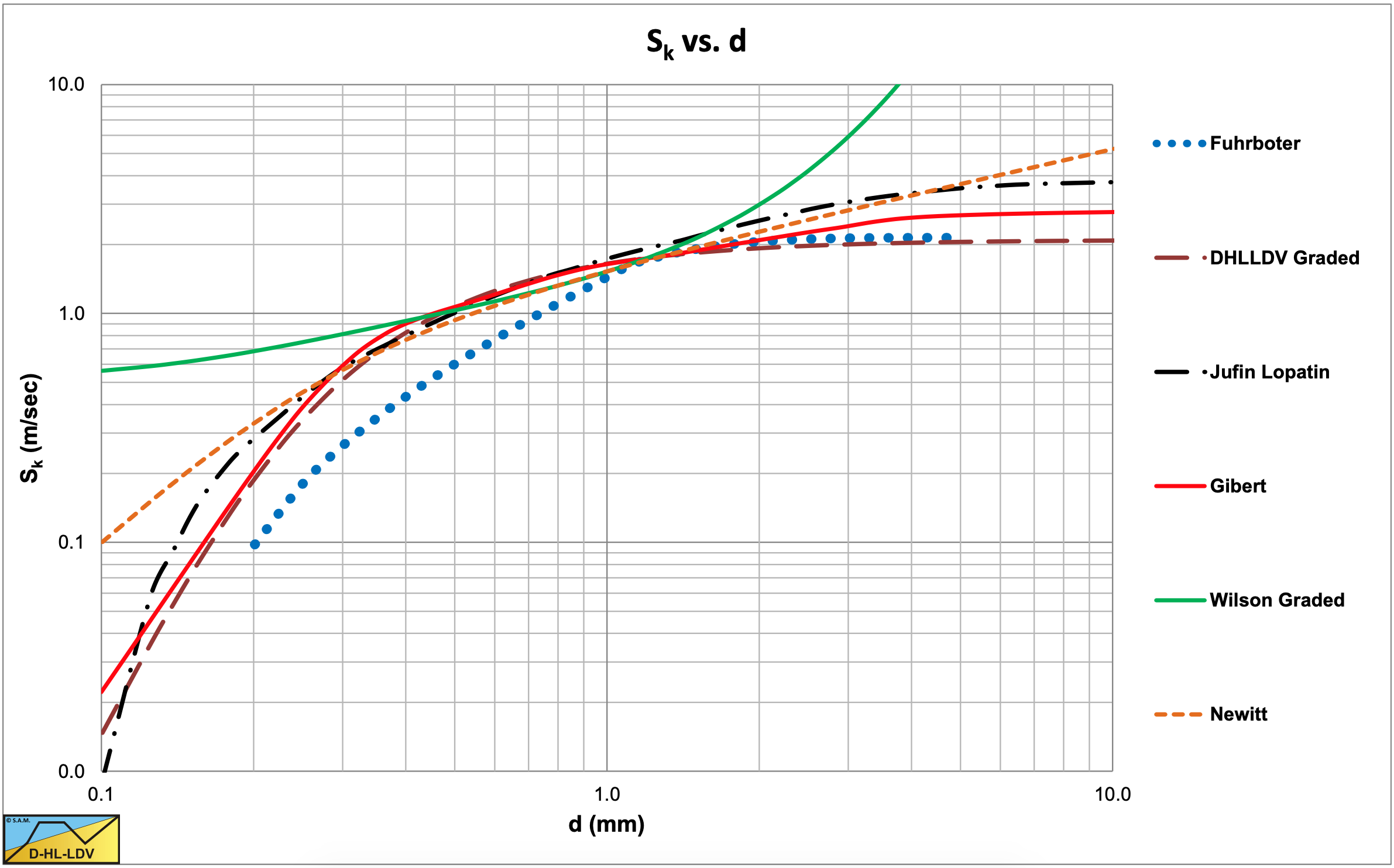
Table 6.16-1 shows the powers of the different parameters in the S_k equations. Figure 6.16-1, Figure 6.16-2, Figure 6.16-3 and Figure 6.16-4 show the values of S_k for 4 different pipe diameters.

Table 6.16-1: The powers of the different parameters, comparing models.

	Rsd	\(\ v_{\mathrm{l}}\cdot \mathrm{g}\)	g·Dp	√Cx	vls	Cvt	vt	d50
Durand & Condolios	1.5	0.167	0.328	-2.67	-0.155	0.0	0.0	0.00
Newitt et al.	1.0	0.167	-0.172	0.00	-0.155	0.0	1.0	0.00
Fuhrboter	0.0	0.000	0.000	0.00	0.000	0.0	1.0	0.00
Jufin & Lopatin	0.5	0.833	-0.672	-0.75	-0.155	-0.5	0.0	0.00
Wilson et al.	1.45	0.250	0.000	0.00	0.000	0.0	0.0	0.35
DHLLDV	1.0	0.250	0.086	-2.67	0.078	0.0	0.0	0.00

For a pipe diameter of D_p=0.1016 m (4 inch) the curves are close together for medium and coarse sands. Wilson, Newitt and Jufin-Lopatin give higher values for the fines, while Wilson and Newitt also give higher values for the coarse particles. The latter can be explained by the fact that both have a sliding bed model for coarser particles. Fuhrboter gives relatively small values for medium sands.

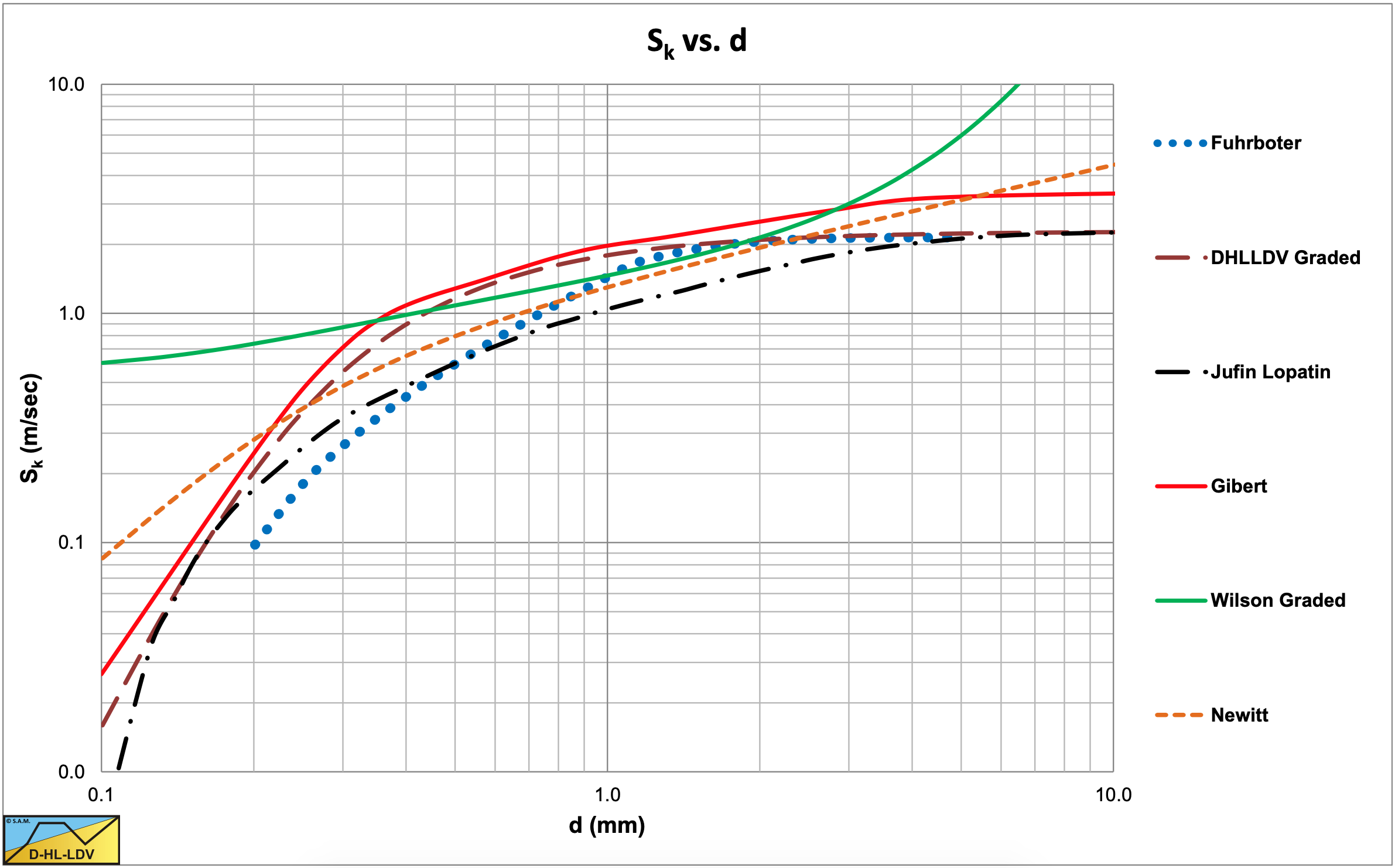
For a pipe diameter of D_p=0.2032 m (8 inch) the curves are not too far apart for medium and coarse sands, but further apart compared to the D_p=0.1016 m pipe. The Wilson curve is less steep.

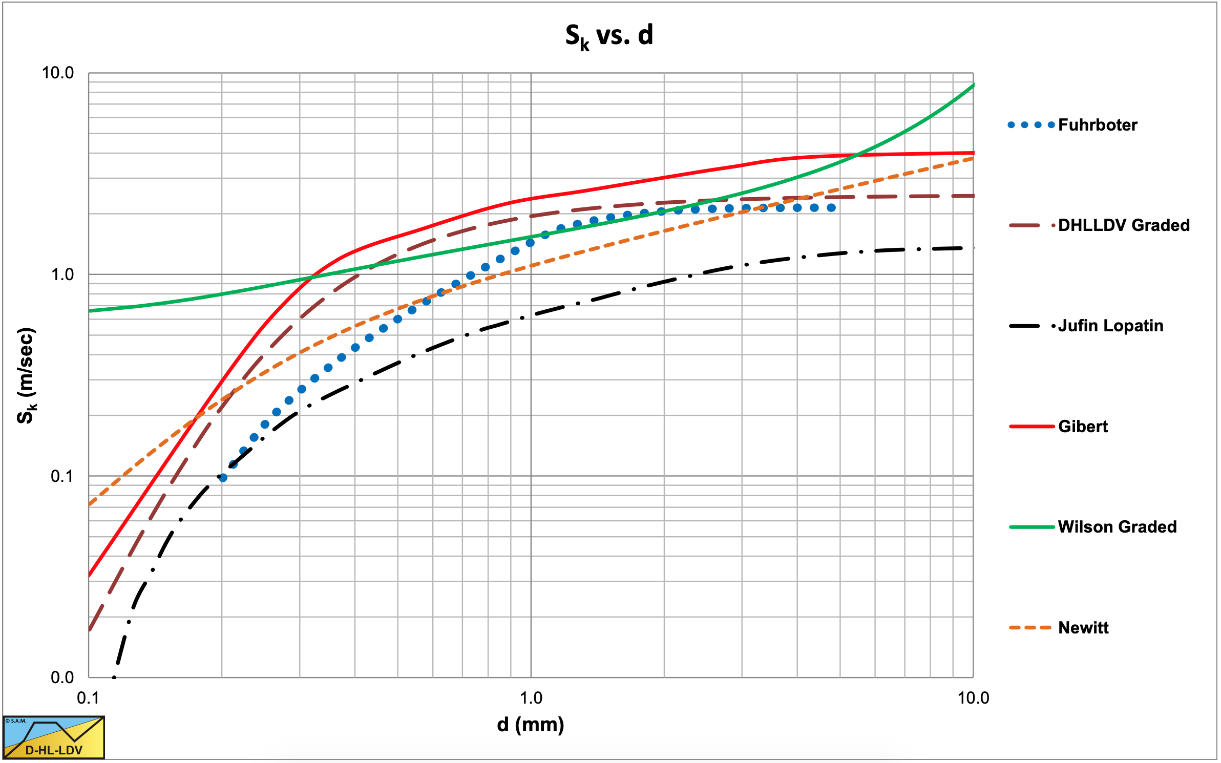
For a pipe diameter of D_p=0.4064 m (16 inch), the curves deviate more. The Wilson curve is less steep again and the Jufin-Lopatin curve is lowering.

For a pipe diameter of D_p=0.8132 m (32 inch), the curves deviate even more. For all pipe diameters the DHLLDV Framework and the Wilson model match very well for particles around d=0.8 mm and the DHLLDV Framework matches well with the Fuhrboter model for particles with d>1 mm.

Figure 6.16-1: The Sk value of 6 models for D_p=0.1016 m, v_ls=3 m/s and C_vt=0.2.

Figure 6.16-2 The Sk value of 6 models for D_p=0.2032 m, v_ls=4 m/s and C_vt=0.2.

Figure 6.16-3 The Sk value of 6 models for D_p=0.4064 m, v_ls=5 m/s and C_vt=0.2.

Figure 6.16-4 The Sk value of 6 models for D_p=0.8132 m, v_ls=6 m/s and C_vt=0.2.

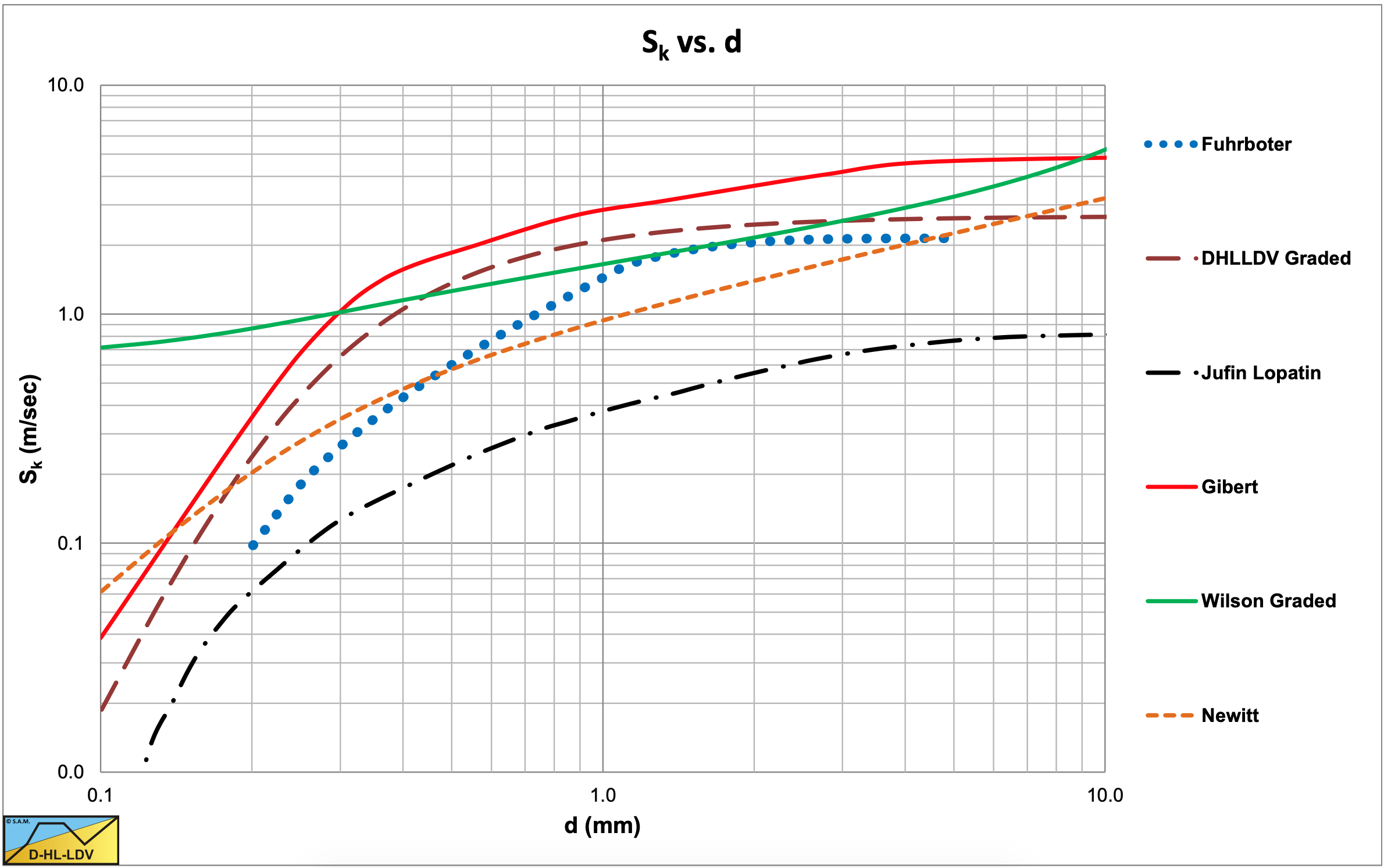
It should be mentioned that the Jufin-Lopatin model depends on the concentration, while all other models don’t. Since most models are based on experiments with small pipe diameters and medium sands, the tendencies found are no surprise. With small pipe diameters and medium sands the models are very close and the differences will fall within the range of the scatter.

6.16.4 Sliding Bed Regime

For the sliding bed regime 4 models are chosen for comparison, the Newitt et al. (1955) model, the Babcock (1970) model and the Yagi et al. (1972) models for sand and gravel. The first two models consider delivered volumetric concentration experiments, the last two spatial concentration experiments.

Below the Limit Deposit Velocity Newitt et al. (1955) found for a sliding bed in a 1 inch steel pipe:

\[\ \mathrm{i}_{\mathrm{m}}=\mathrm{i}_{\mathrm{l}} \cdot\left(\mathrm{1}+\mathrm{6 6} \cdot\left(\mathrm{g} \cdot \mathrm{D}_{\mathrm{p}} \cdot \mathrm{R}_{\mathrm{s d}}\right) \cdot \mathrm{C}_{\mathrm{v t}} \cdot\left(\frac{\mathrm{1}}{\mathrm{v}_{\mathrm{l s}}}\right)^{2}\right)\]

Or:

\[\ \mathrm{i}_{\mathrm{m}}=\mathrm{i}_{\mathrm{l}}+\mathrm{3 3} \cdot \lambda_{\mathrm{l}} \cdot \mathrm{R}_{\mathrm{s d}} \cdot \mathrm{C}_{\mathrm{v t}}\]

Substituting the Darcy-Weisbach friction factor equation and a 1 inch pipe diameter, this gives:

\[\ \mathrm{i}_{\mathrm{m}}=\mathrm{i}_{\mathrm{l}}+\mathrm{0 . 7 5 6} \cdot \mathrm{R}_{\mathrm{s d}} \cdot \mathrm{C}_{\mathrm{v} \mathrm{t}} \cdot\left(\mathrm{v}_{\mathrm{l s}}\right)^{-\mathrm{0 . 1 5 5}}\]

Showing a slight decrease of the solids effect with increasing line speed, as was found by Newitt et al. (1955).

Below the Limit Deposit Velocity Babcock (1970) found for a sliding bed in a 1 inch plastic pipe:

\[\ \mathrm{i}_{\mathrm{m}}=\mathrm{i}_{\mathrm{l}} \cdot\left(\mathrm{1}+\mathrm{6 0 . 6} \cdot\left(\mathrm{g} \cdot \mathrm{D}_{\mathrm{p}} \cdot \mathrm{R}_{\mathrm{s d}}\right) \cdot \mathrm{C}_{\mathrm{v} \mathrm{t}} \cdot\left(\frac{\mathrm{1}}{\mathrm{v}_{\mathrm{l s}}}\right)^{2}\right)\]

Or:

\[\ \mathrm{i}_{\mathrm{m}}=\mathrm{i}_{\mathrm{l}}+\mathrm{3} \mathrm{0} . \mathrm{3} \cdot \lambda_{\mathrm{l}} \cdot \mathrm{R}_{\mathrm{s d}} \cdot \mathrm{C}_{\mathrm{v t}}\]

Substituting the Darcy-Weisbach friction factor equation and a 1 inch pipe diameter, this gives:

\[\ \mathrm{i}_{\mathrm{m}}=\mathrm{i}_{\mathrm{l}}+\mathrm{0 . 6 9 4} \cdot \mathrm{R}_{\mathrm{s d}} \cdot \mathrm{C}_{\mathrm{v t}} \cdot\left(\mathrm{v}_{\mathrm{l s}}\right)^{-\mathrm{0 . 1 5 5}}\]

In both cases the delivered volumetric concentration was used, meaning that the spatial volumetric concentration was larger, especially with a sliding bed. In both models, the solids effect in the hydraulic gradient depends slightly on the cross section averaged line speed.

Below the Limit Deposit Velocity Yagi et al. (1972) found for a sliding bed in different pipes:

For sand ψ<3 (below LDV):

\[\ \frac{\mathrm{i}_{\mathrm{m}}-\mathrm{i}_{\mathrm{l}}}{\mathrm{i}_{\mathrm{l}} \cdot \mathrm{C}_{\mathrm{v s}}}=\Phi=\mathrm{K} \cdot \Psi^{-1.55} \quad\text{ with: }\quad \mathrm{K}=\mathrm{1 0 0}\]

For gravel ψ<3 (below LDV):

\[\ \frac{\mathrm{i}_{\mathrm{m}}-\mathrm{i}_{\mathrm{l}}}{\mathrm{i}_{\mathrm{l}} \cdot \mathrm{C}_{\mathrm{v s}}}=\Phi=\mathrm{K} \cdot \Psi^{-1.16} \quad\text{ with: }\quad \mathrm{K}=\mathrm{9 8}\]

With:

\[\ \Psi=\left(\frac{\mathrm{v}_{\mathrm{l s}}^{2}}{\mathrm{g} \cdot \mathrm{D}_{\mathrm{p}} \cdot \mathrm{R}_{\mathrm{s d}}}\right) \cdot \sqrt{\mathrm{C}_{\mathrm{x}}}\]

This gives:

For sand ψ<3 (below LDV):

\[\ \mathrm{i}_{\mathrm{m}}=\mathrm{i}_{\mathrm{l}}+\mathrm{5 0} \cdot \lambda_{\mathrm{l}} \cdot\left(\mathrm{g} \cdot \mathrm{D}_{\mathrm{p}}\right)^{0.55} \cdot \mathrm{R}_{\mathrm{s d}}^{\mathrm{1 . 5 5}} \cdot\left(\frac{\mathrm{1}}{\sqrt{\mathrm{C}_{\mathrm{x}}}}\right)^{1.55} \cdot \frac{\mathrm{1}}{\mathrm{v}_{\mathrm{l} \mathrm{s}}^{\mathrm{1 . 1}}} \cdot \mathrm{C}_{\mathrm{v} \mathrm{s}}\]

For gravel ψ<3 (below LDV):

\[\ \mathrm{i}_{\mathrm{m}}=\mathrm{i}_{\mathrm{l}}+\mathrm{4} \mathrm{9} \cdot \lambda_{\mathrm{l}} \cdot\left(\mathrm{g} \cdot \mathrm{D}_{\mathrm{p}}\right)^{0.16} \cdot\left(\frac{\mathrm{1}}{\sqrt{\mathrm{C}_{\mathrm{x}}}}\right)^{1.16} \cdot \mathrm{R}_{\mathrm{s d}}^{\mathrm{1 . 1 6}} \cdot \frac{\mathrm{1}}{\mathrm{v}_{\mathrm{l} \mathrm{s}}^{\mathrm{0 . 3 2}}} \cdot \mathrm{C}_{\mathrm{v} \mathrm{s}}\]

Substitution of the Darcy-Weisbach friction factor, a fixed value of 0.6 for √C_x and a fixed value of 1.65 for the relative submerged density, this gives:

\[\ \mathrm{i}_{\mathrm{m}}=\mathrm{i}_{\mathrm{l}}+\mathrm{1.66} \cdot \mathrm{R}_{\mathrm{s d}} \cdot \mathrm{C}_{\mathrm{v s}} \cdot \frac{\mathrm{1}}{\mathrm{v}_{\mathrm{l} \mathrm{s}}^{\mathrm{0 . 4 7 5}}}\]

With an average line speeds around 5 m/sec, this can be reduced to:

\[\ \mathrm{i}_{\mathrm{m}}=\mathrm{i}_{\mathrm{l}}+\mathrm{0 . 7 7} \cdot \mathrm{R}_{\mathrm{s d}} \cdot \mathrm{C}_{\mathrm{v s}}\]

This would imply a high sliding friction factor of 0.83, which was already remarked in the chapter about Yagi et al. (1972). Normally this sliding friction factor has a value in the range 0.35-0.45. The Yagi et al. (1972) equations are based on spatial volumetric concentration, while the Newitt et al. (1955) and Babcock (1970) measurements are based on delivered volumetric concentration. It should be mentioned however that the Newitt et al. (1955) data also show a decreasing solids effect with increasing line speed, but Newitt et al. (1955) just took the average solids effect value. The Yagi et al. (1972) equation for sand is very similar to the Durand & Condolios (1952) equation for heterogeneous transport, which could be expected based on the conclusions of Durand & Condolios (1952).

6.16.5 Homogeneous Regime

The only scientific equation (and explanation) found for the homogeneous regime was derived by Talmon (2011) & (2013), with α_h=6.7:

\[\ \mathrm{i}_{\mathrm{m}}=\mathrm{i}_{\mathrm{l}} \cdot \frac{\mathrm{1}+\mathrm{R}_{\mathrm{s d}} \cdot \mathrm{C}_{\mathrm{v s}}}{\left(\alpha_{\mathrm{h}} \cdot \sqrt{\frac{\lambda_{\mathrm{l}}}{\mathrm{8}}}{ \cdot \mathrm{R}_{\mathrm{s d}} \cdot \mathrm{C}_{\mathrm{v s}}+\mathrm{1}}\right)^{2}}\]

This equation reduces the solids effect compared to the ELM. In some cases it may be necessary to use the Thomas (1965) viscosity to correct for high concentration fines. Others mention a reduction of the solids effect to 60% or even to zero, but no explanation is given.

6.16.6 Validation

To validate the conclusions, independent experiments are considered. Wiedenroth (1967) carried out experiments in a D_p=0.125 m pipe with fine sand, coarse sand, fine gravel and medium gravel. All experiments were carried out with constant spatial volumetric concentration. Figure 6.16-5 shows the results of fine sand. The heterogeneous and homogeneous flow regimes can be recognized. The theoretical DHLLDV Framework curve contains the influence of grading and the Thomas (1965) viscosity.

Figure 6.16-5: Experiments of Wiedenroth (1967) with fine sand, C_vs.

Including the Thomas (1965) viscosity.

Figure 6.16-6: Experiments of Wiedenroth (1967) with coarse sand, C_vs.

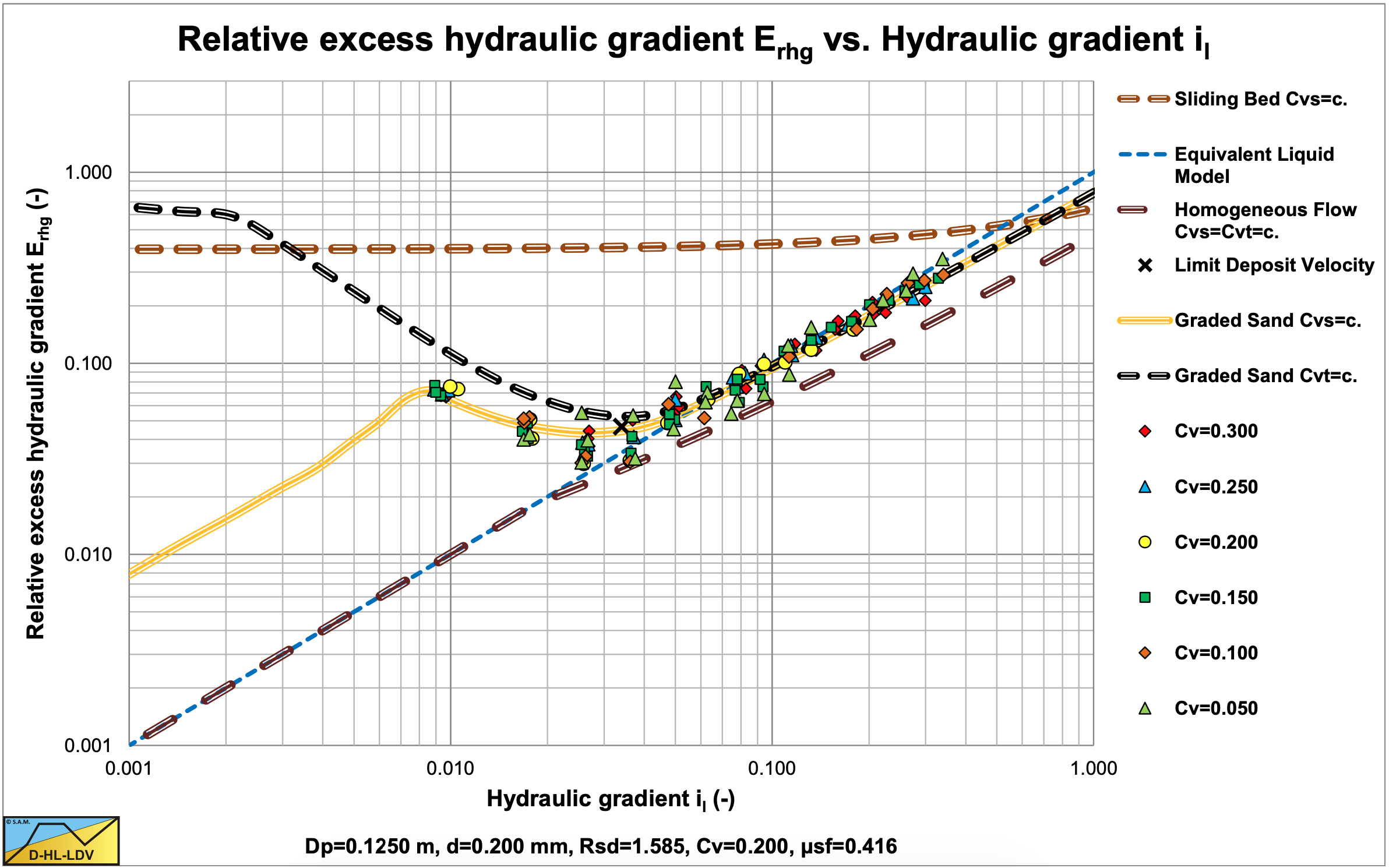
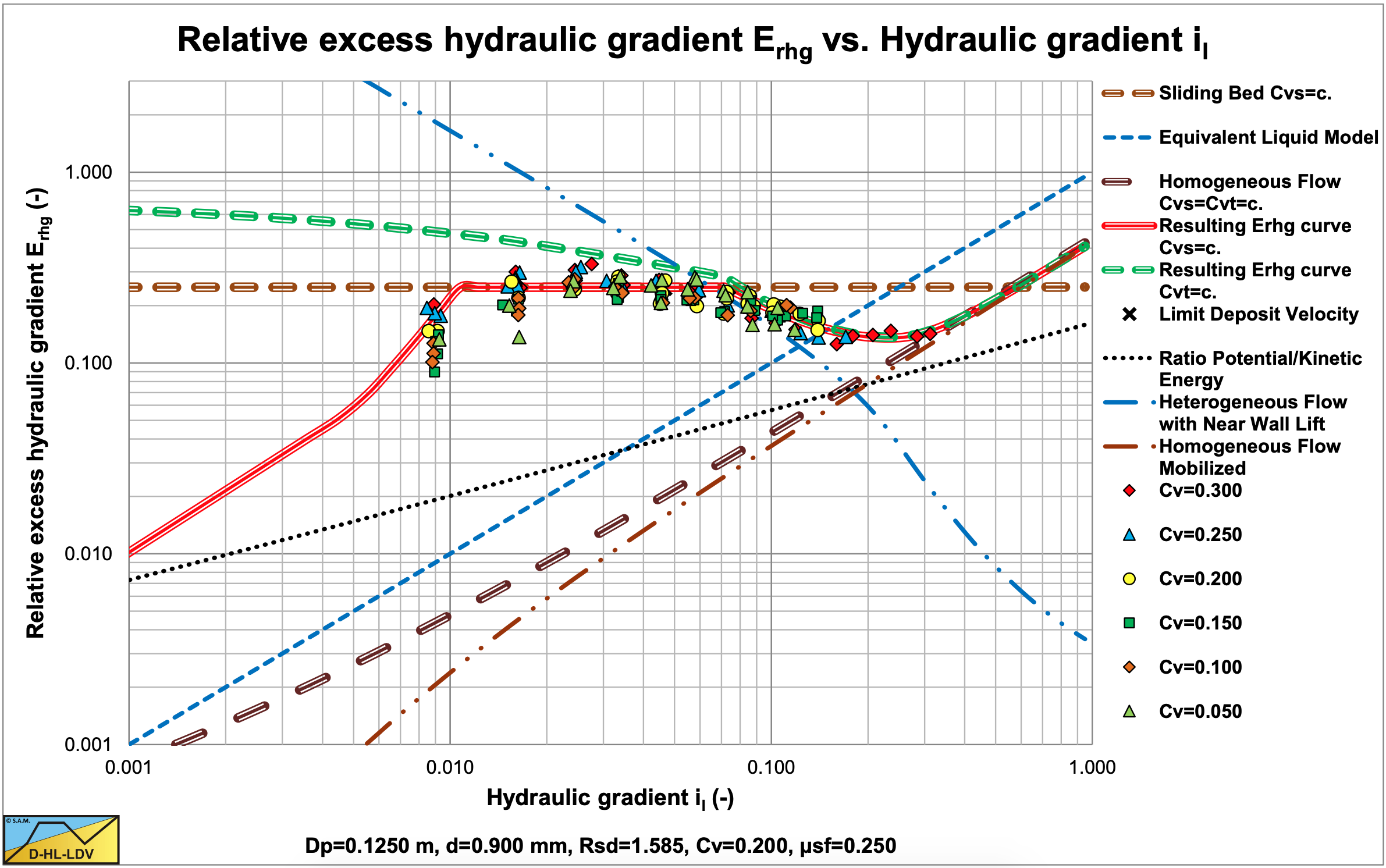
Figure 6.16-6 shows the results for coarse sand. The fixed/stationary bed regime, the sliding bed regime and the start of the heterogeneous regime can be recognized. The influence of the volumetric concentration can hardly be identified in the scatter of data points, meaning that the E_rhg value is independent of the C_vs value.

Figure 6.16-7: Experiments of Wiedenroth (1967) with fine gravel, C_vs.

Figure 6.16-8: Experiments of Wiedenroth (1967) with medium gravel, C_vs.

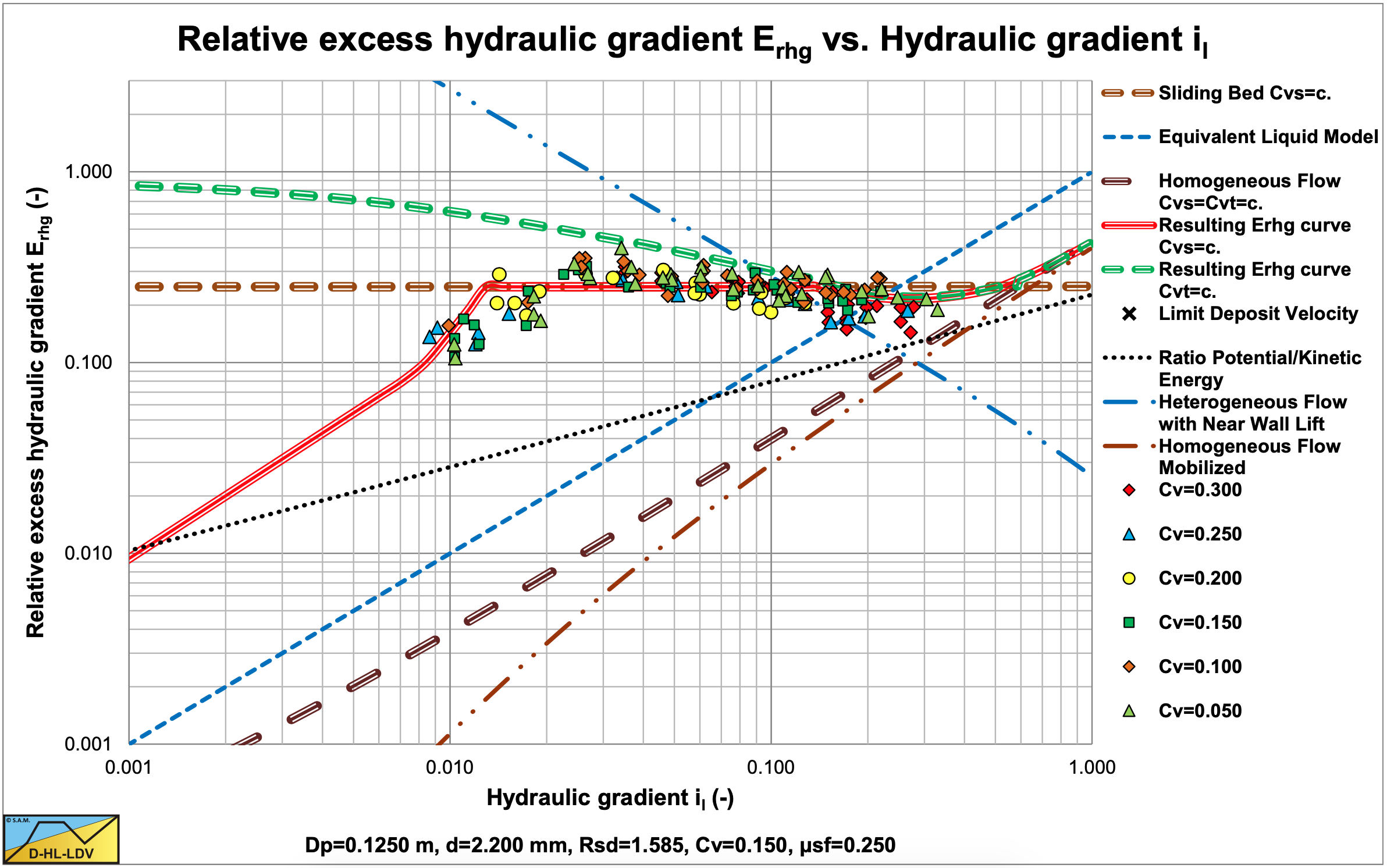
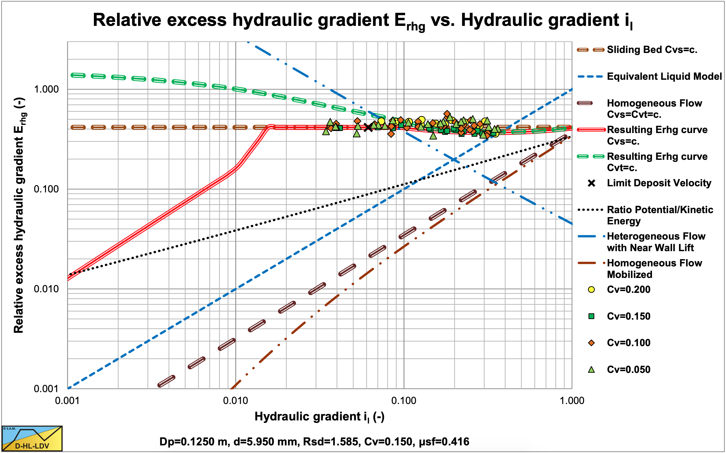
Figure 6.16-7 shows the results for fine gravel. The fixed/stationary bed, the sliding bed and sliding flow can be distinguished. The data points for high line speeds are in between the heterogeneous and the sliding bed curves. This behavior is identified as sliding flow.
Figure 6.16-8 shows the results for medium gravel. Here the sliding bed and sliding flow regimes can be distinguished. However the particles are so large compared to the pipe diameter, that sliding flow and sliding bed almost have the same behavior.