7.14: Inclined Pipes

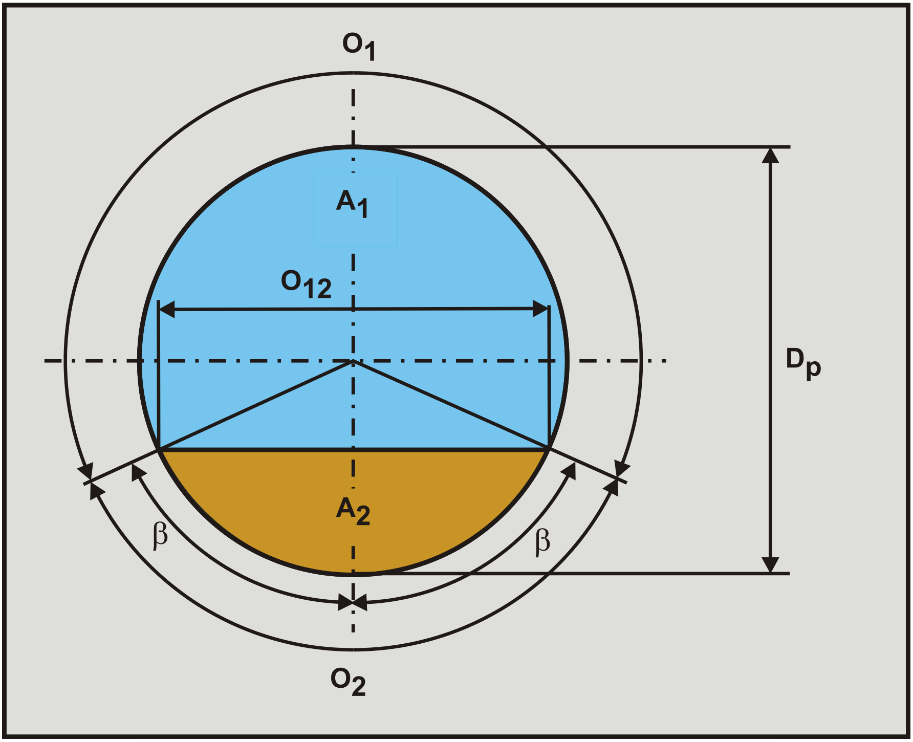
In dredging and other industries often parts of a pump/pipeline system are inclined or vertical. So it is interesting to see what the implications of an inclined pipe on the pressure losses are. This chapter gives an analytical solution to this problem. Figure 7.14-1 shows the definitions of perimeters and cross sections of the pipe.

Figure 7.14-1: Definitions.

7.14.1 Pure Carrier Liquid

First of all, the flow of pure carrier liquid. The perimeter O=O₁ for β=0 in the case of zero concentration. The equilibrium of forces on the liquid in a pipe with inclination angle θ is:

\[\ -\frac{\mathrm{d p}}{\mathrm{d x}} \cdot \mathrm{A} \cdot \mathrm{L}=\tau_{\mathrm{l}} \cdot \mathrm{O} \cdot \mathrm{L}+\rho_{\mathrm{l}} \cdot \mathrm{A} \cdot \mathrm{L} \cdot \mathrm{g} \cdot \sin (\theta)\]

The shear stress \(\ \tau_{\mathrm{l}}\) can be determined with the well known Darcy-Weisbach equation.

Figure 7.14-2: Pure carrier liquid in an inclined pipe.

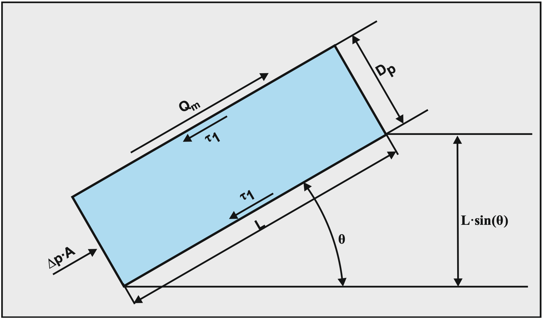
Figure 7.14-2 shows the driving force and resisting shear stresses in the pipe. The shear stress, in general, is defined by, based on the Darcy Weisbach equation:

\[\ \tau=\frac{\lambda_{\mathrm{l}}}{8} \cdot \rho_{\mathrm{l}} \cdot \mathrm{v}_{\mathrm{l s}}^{2}\]

The hydraulic gradient can now be determined with:

\[\ \mathrm{i}_{\mathrm{l}, \theta}=-\frac{\mathrm{d p}}{\mathrm{d x}} \cdot \frac{\mathrm{A} \cdot \mathrm{L}}{\rho_{\mathrm{l}} \cdot \mathrm{A} \cdot \mathrm{L} \cdot \mathrm{g}}=\frac{\tau_{\mathrm{l}} \cdot \mathrm{O} \cdot \mathrm{L}}{\rho_{\mathrm{l}} \cdot \mathrm{A} \cdot \mathrm{L} \cdot \mathrm{g}}+\frac{\rho_{\mathrm{l}} \cdot \mathrm{A} \cdot \mathrm{L} \cdot \mathrm{g} \cdot \sin (\theta)}{\rho_{\mathrm{l}} \cdot \mathrm{A} \cdot \mathrm{L} \cdot \mathrm{g}}=\mathrm{i}_{\mathrm{l}}+\sin (\theta)\]

So apparently the hydraulic gradient increases with the sine of the inclination angle. Which also means that a downwards slope with a negative inclination angle gives a negative sine and thus a reduction of the hydraulic gradient. In this case the total hydraulic gradient may even become negative.

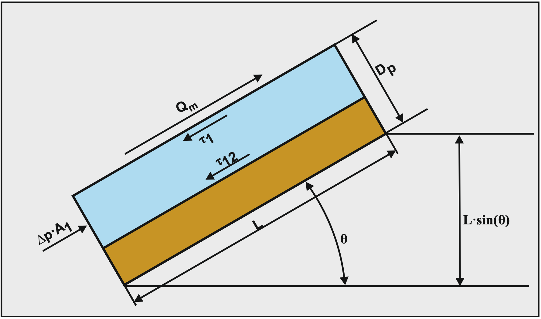
7.14.2 Stationary Bed Regime

The equilibrium of forces on the layer of liquid above the bed is, where Figure 7.14-3 shows the driving force and the resisting shear stresses on the liquid above the bed:

\[\ -\frac{\mathrm{d p}}{\mathrm{d x}} \cdot \mathrm{A}_{1} \cdot \mathrm{L}=\tau_{1} \cdot \mathrm{O}_{1} \cdot \mathrm{L}+\tau_{12} \cdot \mathrm{O}_{12} \cdot \mathrm{L}+\rho_{\mathrm{l}} \cdot \mathrm{A}_{1} \cdot \mathrm{L} \cdot \mathrm{g} \cdot \sin (\theta)\]

Since the bed is not moving, the friction between the bed and the pipe wall compensates for the weight component of the bed. The hydraulic gradient can now be determined with:

\[\ \mathrm{i}_{\mathrm{m}, \theta}=-\frac{\mathrm{d p}}{\mathrm{d x}} \cdot \frac{\mathrm{A}_{1} \cdot \mathrm{L}}{\rho_{\mathrm{l}} \cdot \mathrm{A}_{1} \cdot \mathrm{L} \cdot \mathrm{g}}=\frac{\tau_{1} \cdot \mathrm{O}_{1} \cdot \mathrm{L}+\tau_{12} \cdot \mathrm{O}_{12} \cdot \mathrm{L}}{\rho_{\mathrm{l}} \cdot \mathrm{A}_{1} \cdot \mathrm{L} \cdot \mathrm{g}}+\sin (\theta)=\mathrm{i}_{\mathrm{m}}+\sin (\theta)\]

Which is the hydraulic gradient of a stationary bed in horizontal pipe plus the sine of the inclination angle. The weight of the solids do not give a contribution to the hydraylic gradient.

Figure 7.14-3: The stationary bed regime in an inclined pipe.

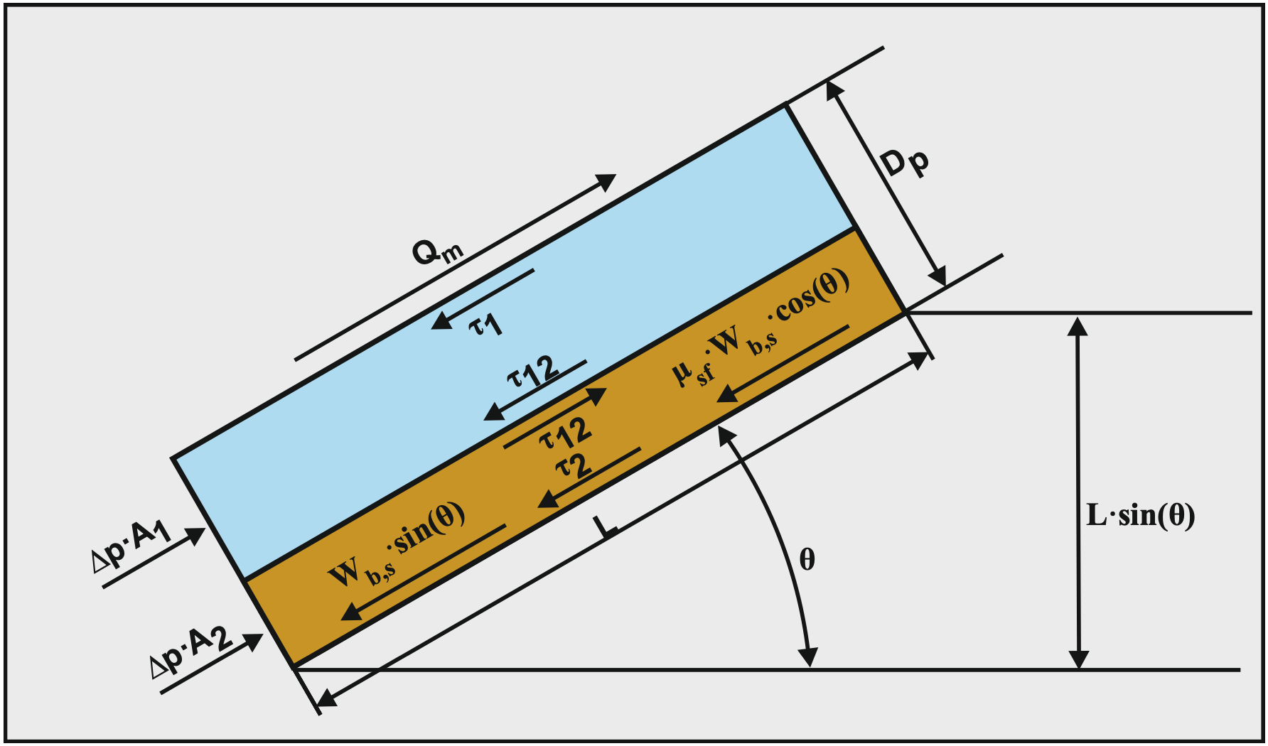
7.14.3 Sliding Bed Regime

The equilibrium of forces on the layer of liquid above the bed is:

\[\ -\frac{\mathrm{dp}}{\mathrm{dx}} \cdot \mathrm{A}_{1} \cdot \mathrm{L}=\tau_{1} \cdot \mathrm{O}_{1} \cdot \mathrm{L}+\tau_{12} \cdot \mathrm{O}_{12} \cdot \mathrm{L}+\rho_{\mathrm{l}} \cdot \mathrm{A}_{1} \cdot \mathrm{L} \cdot \mathrm{g} \cdot \sin (\theta)\]

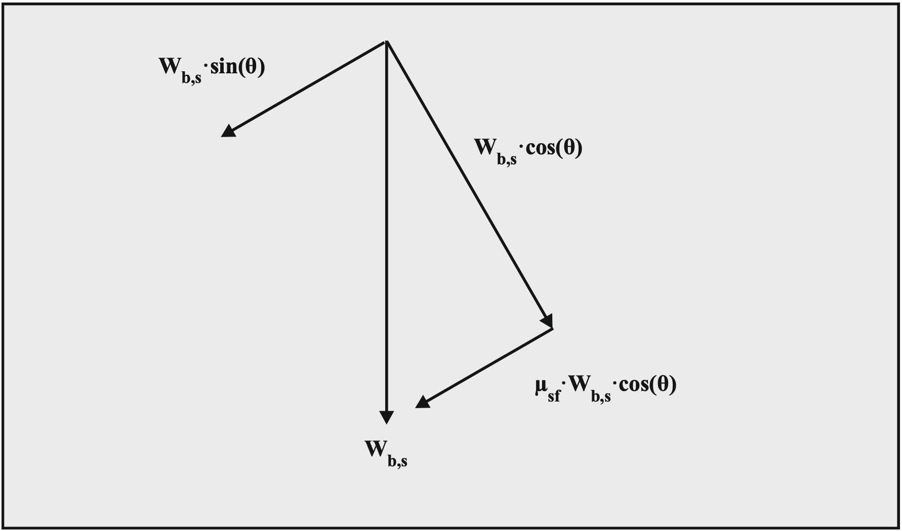
Figure 7.14-4 shows how the submerged weight of the bed results in a resisting force, a normal force on the pipe wall and a sliding friction force between the bed and the pipe wall. Figure 7.14-5 shows the driving forces and resisting forces and shear stresses, both on the liquid above the bed and on the bed.

The cross-section of the bed can be determined with:

\[\ \mathrm{A}_{2}=\frac{\mathrm{C}_{\mathrm{v} \mathrm{s}}}{\mathrm{C}_{\mathrm{v} \mathrm{b}}} \cdot \mathrm{A}\]

The weight of the bed, including pore water is:

\[\ \begin{array}{left} \mathrm{w}_{\mathrm{b}} &=\rho_{\mathrm{b}} \cdot \mathrm{A}_{\mathrm{2}} \cdot \mathrm{L} \cdot \mathrm{g}=\left(\rho_{\mathrm{s}} \cdot \mathrm{C}_{\mathrm{v} \mathrm{b}}+\rho_{\mathrm{l}} \cdot\left(\mathrm{1}-\mathrm{C}_{\mathrm{v} \mathrm{b}}\right)\right) \cdot \mathrm{A}_{2} \cdot \mathrm{L} \cdot \mathrm{g} \\ &=\left(\left(\rho_{\mathrm{s}}-\rho_{\mathrm{l}}\right) \cdot \mathrm{C}_{\mathrm{v} \mathrm{b}}+\rho_{\mathrm{l}}\right) \cdot \mathrm{A}_{2} \cdot \mathrm{L} \cdot \mathrm{g}=\rho_{\mathrm{l}} \cdot \mathrm{R}_{\mathrm{s d}} \cdot \mathrm{C}_{\mathrm{v s}} \cdot \mathrm{A} \cdot \mathrm{L} \cdot \mathrm{g}+\rho_{\mathrm{l}} \cdot \mathrm{A}_{2} \cdot \mathrm{L} \cdot \mathrm{g} \end{array}\]

The submerged weight of the bed can be determined with:

\[\ \mathrm{W}_{\mathrm{b}, \mathrm{s}}=\left(\rho_{\mathrm{s}}-\rho_{\mathrm{l}}\right) \cdot \mathrm{C}_{\mathrm{v} \mathrm{b}} \cdot \mathrm{A}_{\mathrm{2}} \cdot \mathrm{L} \cdot \mathrm{g}=\rho_{\mathrm{l}} \cdot \mathrm{R}_{\mathrm{s d}} \cdot \mathrm{C}_{\mathrm{v s}} \cdot \mathrm{A} \cdot \mathrm{L} \cdot \mathrm{g}\]

This gives for the equilibrium of forces on the bed:

\[\ \begin{array}{left} -\frac{\mathrm{d p}}{\mathrm{d x}} \cdot \mathrm{A}_{2} \cdot \mathrm{L}=\tau_{2} \cdot \mathrm{O}_{2} \cdot \mathrm{L}-\tau_{12} \cdot \mathrm{O}_{12} \cdot \mathrm{L}+\mathrm{W}_{\mathrm{b}} \cdot \sin (\theta)+\mu_{\mathrm{s f}} \cdot \mathrm{W}_{\mathrm{b}, \mathrm{s}} \cdot \cos (\theta)\\
-\frac{\mathrm{d p}}{\mathrm{d x}} \cdot \mathrm{A}_{2} \cdot \mathrm{L}=\tau_{2} \cdot \mathrm{O}_{2} \cdot \mathrm{L}-\tau_{12} \cdot \mathrm{O}_{12} \cdot \mathrm{L}+\mathrm{W}_{\mathrm{b}, \mathrm{s}} \cdot \sin (\theta)+\mu_{\mathrm{s f}} \cdot \mathrm{W}_{\mathrm{b}, \mathrm{s}} \cdot \cos (\theta)+\rho_{\mathrm{l}} \cdot \mathrm{A}_{2} \cdot \mathrm{L} \cdot \mathrm{g} \cdot \sin (\theta)\end{array}\]

For the whole pipe cross section the two contributions can be added, giving:

\[\ \begin{array}{left}-\frac{\mathrm{d p}}{\mathrm{d x}} \cdot \mathrm{A} \cdot \mathrm{L}=& \tau_{1} \cdot \mathrm{O}_{1} \cdot \mathrm{L}+\tau_{2} \cdot \mathrm{O}_{2} \cdot \mathrm{L}+\rho_{\mathrm{l}} \cdot \mathrm{A} \cdot \mathrm{L} \cdot \mathrm{g} \cdot \sin (\theta) \\ &+\rho_{\mathrm{l}} \cdot \mathrm{R}_{\mathrm{s d}} \cdot \mathrm{C}_{\mathrm{v s}} \cdot \mathrm{A} \cdot \mathrm{L} \cdot \mathrm{g} \cdot \sin (\theta)+\mu_{\mathrm{s f}} \cdot \rho_{\mathrm{l}} \cdot \mathrm{R}_{\mathrm{s} \mathrm{d}} \cdot \mathrm{C}_{\mathrm{v s}} \cdot \mathrm{A} \cdot \mathrm{L} \cdot \mathrm{g} \cdot \mathrm{c o s}(\theta) \end{array}\]

This can also be written as:

\[\ -\frac{\mathrm{d p}}{\mathrm{d x}} \cdot \mathrm{A} \cdot \mathrm{L}=\tau_{1} \cdot \mathrm{O}_{1} \cdot \mathrm{L}+\tau_{2} \cdot \mathrm{O}_{2} \cdot \mathrm{L}+\rho_{\mathrm{m}} \cdot \mathrm{A} \cdot \mathrm{L} \cdot \mathrm{g} \cdot \sin (\theta)+\mu_{\mathrm{s f}} \cdot \rho_{\mathrm{l}} \cdot \mathrm{R}_{\mathrm{s d}} \cdot \mathrm{C}_{\mathrm{v s}} \cdot \mathrm{A} \cdot \mathrm{L} \cdot \mathrm{g} \cdot \cos (\theta)\]

In terms of the hydraulic gradient this gives:

\[\ \mathrm{i}_{\mathrm{m}, \mathrm{\theta}} =-\frac{\mathrm{d p}}{\mathrm{d} \mathrm{x}} \cdot \frac{\mathrm{A} \cdot \mathrm{L}}{\rho_{\mathrm{l}} \cdot \mathrm{g} \cdot \mathrm{L} \cdot \mathrm{A}}=\frac{\tau_{1} \cdot \mathrm{O}_{1} \cdot \mathrm{L}+\tau_{2} \cdot \mathrm{O}_{2} \cdot \mathrm{L}}{\rho_{\mathrm{l}} \cdot \mathrm{g} \cdot \mathrm{L} \cdot \mathrm{A}}+\left(\mathrm{1}+\mathrm{R}_{\mathrm{s d}} \cdot \mathrm{C}_{\mathrm{v} \mathrm{s}}\right) \cdot \sin (\theta) +\mu_{\mathrm{s f}} \cdot \mathrm{R}_{\mathrm{s d}} \cdot \mathrm{C}_{\mathrm{v} \mathrm{s}} \cdot \cos (\theta) \]

In chapter 7.4 it has been proven that the first term on the right hand side almost equals the pure liquid hydraulic gradient i_l, without pipe inclination, so:

\[\ \begin{array}{left}\mathrm{i}_{\mathrm{m}, \mathrm{\theta}}=\mathrm{i}_{\mathrm{l}}+\left(\mathrm{1}+\mathrm{R}_{\mathrm{s d}} \cdot \mathrm{C}_{\mathrm{v s}}\right) \cdot \sin (\theta)+\mu_{\mathrm{s f}} \cdot \mathrm{R}_{\mathrm{s d}} \cdot \mathrm{C}_{\mathrm{v s}} \cdot \cos (\theta)\\
\mathrm{i}_{\mathrm{m}, \mathrm{\theta}}=\left(\mathrm{i}_{\mathrm{l}}+\sin (\theta)\right)+\mathrm{R}_{\mathrm{s d}} \cdot \mathrm{C}_{\mathrm{v s}} \cdot\left(\mu_{\mathrm{s f}} \cdot \cos (\theta)+\sin (\theta)\right)\end{array}\]

The hydraulic gradient for pure liquid with pipe inclination can now be expressed as:

\[\ \mathrm{i}_{\mathrm{l}, \theta}=\mathrm{i}_{\mathrm{l}}+\sin (\theta)\]

Figure 7.14-4: The submerged weight components and the sliding friction force.

Giving for the mixture hydraulic gradient with pipe inclination:

\[\ \mathrm{i}_{\mathrm{m}, \mathrm{\theta}}=\mathrm{i}_{\mathrm{l}, \theta}+\mathrm{R}_{\mathrm{s d}} \cdot \mathrm{C}_{\mathrm{v s}} \cdot\left(\mu_{\mathrm{s f}} \cdot \cos (\theta)+\sin (\theta)\right)\]

The relative excess hydraulic gradient E_rhg,θ is now:

\[\ \mathrm{E}_{\mathrm{r h g}, \theta}=\frac{\mathrm{i}_{\mathrm{m}, \mathrm{\theta}}-\mathrm{i}_{\mathrm{l}, \mathrm{\theta}}}{\mathrm{R}_{\mathrm{s d}} \cdot \mathrm{C}_{\mathrm{v s}}}=\mu_{\mathrm{s f}} \cdot \cos (\theta)+\sin (\theta)\]

Figure 7.14-5: A sliding bed in an inclined pipe.

Apparently the mixture hydraulic gradient in a sliding bed flow regime does not depend on the velocity of the sliding bed. As soon as the bed starts sliding, the above equations are valid. The above equations match the assumption that the solids effect has to be multiplied by the cosine of the inclination angle to a power of 1. This is in accordance with the Worster & Denny (1955) assumptions. The powers of 1.5 by Durand & Condolios (1952) and 1-1.7 by Wilson et al. (1992) seem to be to high.

7.14.4 Heterogeneous Regime

In the heterogeneous flow regime, the energy losses consist of the potential energy losses and the kinetic energy losses. Figure 7.14-6 shows the change of the angle of attack resulting from an inclination angle. The equation for the total head loss in a horizontal pipe is:

\[\ \begin{array}{left} \mathrm{E}_{\mathrm{rhg}}=\mathrm{S}_{\mathrm{hr}}+\mathrm{S}_{\mathrm{rs}}\\
\mathrm{i}_{\mathrm{m}}=\mathrm{i}_{\mathrm{l}}+\left(\mathrm{S}_{\mathrm{hr}}+\mathrm{S}_{\mathrm{rs}}\right) \cdot \mathrm{R}_{\mathrm{sd}} \cdot \mathrm{C}_{\mathrm{vs}}\end{array}\]

The potential energy contribution of the DHLLDV Framework in a horizontal pipe is:

\[\ \mathrm{S}_{\mathrm{hr}}=\frac{\mathrm{v}_{\mathrm{t}} \cdot\left(\mathrm{1}-\frac{\mathrm{C}_{\mathrm{v s}}}{\mathrm{\kappa}_{\mathrm{C}}}\right)^{\beta}}{\mathrm{v}_{\mathrm{l s}}}\]

The kinetic energy contribution of the DHLLDV Framework in a horizontal pipe is:

\[\ \mathrm{S}_{\mathrm{r s}}=\left(\frac{\mathrm{v}_{\mathrm{s} \mathrm{l}}}{\mathrm{v}_{\mathrm{t}}}\right)^{2}=\mathrm{c} \cdot\left(\frac{\delta_{\mathrm{v}}}{\mathrm{d}}\right)^{2 / 3} \cdot\left(\frac{\mathrm{v}_{\mathrm{t}}}{\mathrm{1 1 . 6} \cdot \mathrm{u}_{*}}\right)^{4 / 3} \cdot\left(\frac{\mathrm{v}_{\mathrm{t}}}{\sqrt{\mathrm{g} \cdot \mathrm{d}}}\right)^{2}\]

In an inclined pipe the effective terminal settling velocity perpendicular to the pipe wall, the terminal settling velocity times the cosine of the inclination angle, gives a potential energy term of:

\[\ \mathrm{S}_{\mathrm{hr}, \theta}=\mathrm{S}_{\mathrm{hr}} \cdot \cos (\theta)=\frac{\mathrm{v}_{\mathrm{t}} \cdot \cos (\theta) \cdot\left(1-\frac{\mathrm{C}_{\mathrm{vs}}}{\mathrm{\kappa}_{\mathrm{C}}}\right)^{\beta}}{\mathrm{v}_{\mathrm{ls}}}\]

For the kinetic energy losses, the angle of attack has to be adjusted in an inclined pipe. The angle of attack is defined as the ratio between the terminal settling velocity component perpendicular to the pipe wall and the resulting velocity at the thickness of the viscous sub layer, giving:

\[\ \mathrm{S}_{\mathrm{r s}, \theta}=\mathrm{c} \cdot\left(\frac{\delta_{\mathrm{v}}}{\mathrm{d}}\right)^{2 / 3} \cdot\left(\frac{\mathrm{v}_{\mathrm{t}} \cdot \cos (\theta)}{\mathrm{1 1 .6 \cdot u}_{*}-\mathrm{v}_{\mathrm{t}} \cdot \sin (\theta)}\right)^{4 / 3} \cdot\left(\frac{\mathrm{v}_{\mathrm{t}}}{\sqrt{\mathrm{g} \cdot \mathrm{d}}}\right)^{2}\]

Figure 7.14-6: Heterogeneous flow in an inclined pipe, the angle of attack.

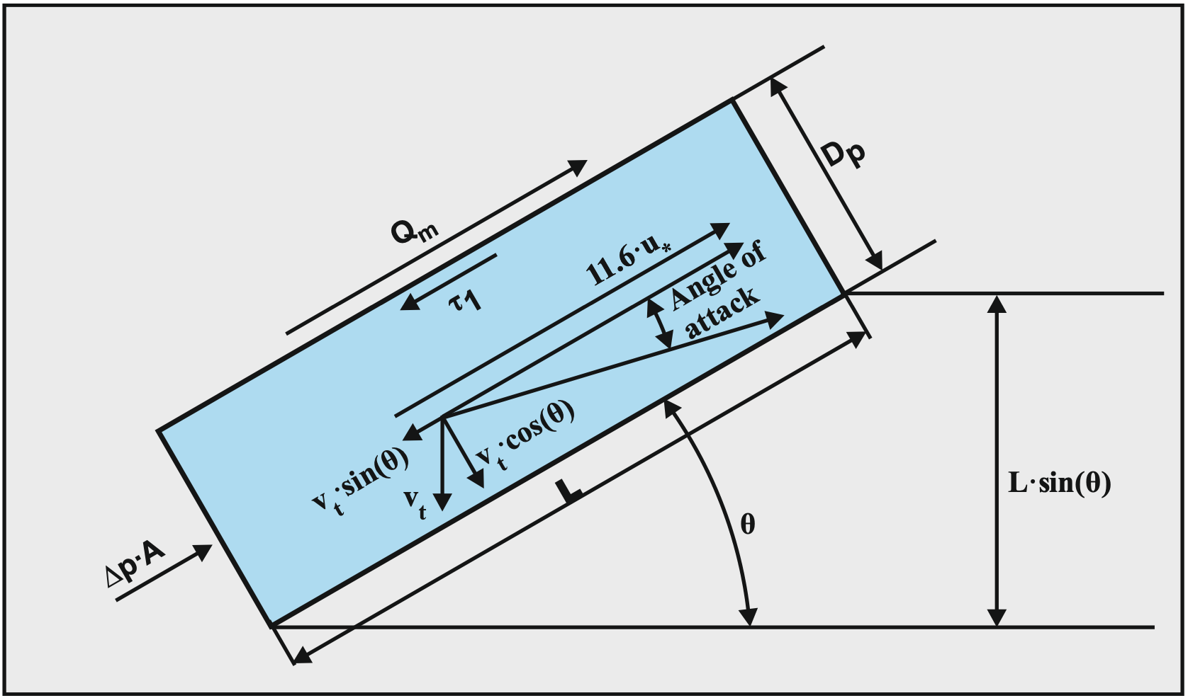
So for very small particles with v_t<<11.6·u*, the kinetic energy losses are proportional to the cosine of the inclination angle to a power of 4/3. For larger particles, the term in the denominator becomes significant resulting in different behavior of a positive versus a negative inclination angle. Apart from this, also the lifting of the mixture has to be added, giving:

\[\ \begin{array}{left}\mathrm{E}_{\mathrm{r h g}, \mathrm{\theta}}=\mathrm{S}_{\mathrm{h r}, \theta}+\mathrm{S}_{\mathrm{r s}, \mathrm{\theta}}+\sin (\theta)\\ \mathrm{i}_{\mathrm{m}, \mathrm{\theta}}=\mathrm{i}_{\mathrm{l}, \theta}+\left(\mathrm{S}_{\mathrm{h r}, \mathrm{\theta}}+\mathrm{S}_{\mathrm{r s}, \mathrm{\theta}}+\sin (\theta)\right) \cdot \mathrm{R}_{\mathrm{s d}} \cdot \mathrm{C}_{\mathrm{v s}}\end{array}\]

Literature (see chapter 6) shows a power of the cosine between 1 and 1.7. Here a more complicated formulation is found. Considering that the potential energy losses are much smaller than the kinetic energy losses, a power of about 4/3 is found for small particles, while larger particles will show a smaller power depending on the terminal settling velocity (see equation (7.14-22)). The higher the terminal settling velocity, the smaller the power. Theoretically this power may even become zero when nominator and denominator decrease in the same way with increasing inclination angle.

7.14.5 Homogeneous Regime

In the homogeneous flow regime the relative excess hydraulic gradient is, including the lubrication effect:

\[\ \begin{array}{left}\mathrm{E}_{\mathrm{r h g}}=\alpha_{\mathrm{E}} \cdot \mathrm{i}_{\mathrm{l}}\\
\mathrm{i}_{\mathrm{m}}=\mathrm{i}_{\mathrm{l}}+\mathrm{i}_{\mathrm{l}} \cdot \mathrm{\alpha}_{\mathrm{E}} \cdot \mathrm{R}_{\mathrm{sd}} \cdot \mathrm{C}_{\mathrm{v s}}=\mathrm{i}_{\mathrm{l}} \cdot\left(1+\alpha_{\mathrm{E}} \cdot \mathrm{R}_{\mathrm{sd}} \cdot \mathrm{C}_{\mathrm{v s}}\right)\end{array}\]

For an inclined pipe only the lifting of the mixture has to be added, giving:

\[\ \begin{array}{left}\mathrm{E}_{\mathrm{rhg}, \theta}&=\alpha_{\mathrm{E}} \cdot \mathrm{i}_{\mathrm{l}}+\sin (\theta)\\ \mathrm{i}_{\mathrm{m}, \theta}&=\mathrm{i}_{\mathrm{l}, \theta}+\left(\alpha_{\mathrm{E}} \cdot \mathrm{i}_{\mathrm{l}}+\sin (\theta)\right) \cdot \mathrm{R}_{\mathrm{sd}} \cdot \mathrm{C}_{\mathrm{vs}}\\ &=\mathrm{i}_{\mathrm{l}} \cdot\left(1+\alpha_{\mathrm{E}} \cdot \mathrm{R}_{\mathrm{sd}} \cdot \mathrm{C}_{\mathrm{vs}}\right)+\sin (\theta) \cdot\left(1+\mathrm{R}_{\mathrm{sd}} \cdot \mathrm{C}_{\mathrm{vs}}\right)\end{array}\]

7.14.6 Sliding Flow Regime

The method for determining the Sliding Flow Regime is not affected by pipe inclination. Of course the equations for a pipe with inclination for the sliding bed regime and the heterogeneous regime have to be applied. However in the Sliding Flow Regime the particles are so large that they do not follow the eddies anymore. The particles will have a slip velocity with respect to the liquid velocity related to the hindered settling velocity and the inclination angle. As a result, the liquid velocity is a bit higher than the cross sectional averaged line speed. The result is a higher hydraulic gradient for the carrier liquid. This gives:

\[\ \begin{array}{left} \mathrm{i}_{\mathrm{m}, \mathrm{\theta}}&=\mathrm{i}_{\mathrm{l}}+\sin (\theta)+\mathrm{i}_{\mathrm{l}} \cdot \frac{\mathrm{2} \cdot \mathrm{v}_{\mathrm{t h}} \cdot \sin (\theta) \cdot \mathrm{C}_{\mathrm{v} \mathrm{s}}}{\mathrm{v}_{\mathrm{l} \mathrm{s}}}+\sin (\theta) \cdot \mathrm{R}_{\mathrm{s d}} \cdot \mathrm{C}_{\mathrm{v} \mathrm{s}}\\ \mathrm{i}_{\mathrm{m}, \mathrm{\theta}}&=\mathrm{i}_{\mathrm{l}, \theta}++\mathrm{i}_{\mathrm{l}} \cdot \frac{\mathrm{2} \cdot \mathrm{v}_{\mathrm{t h}} \cdot \sin (\theta) \cdot \mathrm{C}_{\mathrm{v} \mathrm{s}}}{\mathrm{v}_{\mathrm{l} \mathrm{s}}}+\sin (\theta) \cdot \mathrm{R}_{\mathrm{s} \mathrm{d}} \cdot \mathrm{C}_{\mathrm{v} \mathrm{s}}\\ \mathrm{E}_{\mathrm{r h g}, \mathrm{\theta}}&=\mathrm{i}_{\mathrm{l}} \cdot \frac{\mathrm{2} \cdot \mathrm{v}_{\mathrm{t h}} \cdot \mathrm{s i n}(\theta)}{\mathrm{v}_{\mathrm{l} \mathrm{s}} \cdot \mathrm{R}_{\mathrm{s d}}}+\sin (\theta)\end{array}\]

7.14.7 The Limit Deposit Velocity

The Limit of Stationary Deposit Velocity is affected by the pipe inclination. In an ascending pipe, the cross sectional averaged line speed has to be higher compared to a horizontal pipe in order to make a bed start sliding. In a descending pipe this line speed is lower. It is even possible that in a descending pipe the bed will always slide because of gravity.

The Limit Deposit Velocity is defined as the line speed above which there is no stationary of sliding bed, is determined by either the potential energy losses or a limiting sliding bed. In both cases this is affected by the cosine of the inclination angle, the component of gravity perpendicular to the pipe wall. Since in both cases the Limit Deposit Velocity depends on the cube root of this cosine, the Limit Deposit Velocity will decrease according to:

\[\ \mathrm{v}_{\mathrm{l s}, \mathrm{l d v}, \mathrm{\theta}}=\mathrm{v}_{\mathrm{l s}, \mathrm{l d v}} \cdot \cos (\theta)^{1 / 3}\]

Because of the cube root of this cosine, this means that for angles up to 45o the reduction is less than 10%.

7.14.8 Conclusions & Discussion

For the stationary bed regime, only the potential energy term of the pure liquid has to be added to the hydraulic gradient of the mixture. For all other flow regimes the potential energy term of the mixture has to be added, together with a correction of the so called solids effect. The result of this is a higher line speed for the intersection point of the stationary bed curve and the sliding bed curve. So in general an increase of the Limit of Stationary Deposit Velocity. This may however also result in omission of the occurrence of a sliding bed for an inclined pipe, where a sliding bed would occur in a horizontal pipe. This makes sense, since a higher line speed is required to make a bed start sliding, there is the possibility that the bed is already fully suspended before it could start sliding.

In the sliding bed regime and the heterogeneous regime, the hydraulic gradient is lower for an inclined pipe compared with a horizontal pipe, if the potential energy term of the mixture (static head) is not taken into account, especially for small particles in the heterogeneous regime. For the heterogeneous regime there is a difference between ascending and descending pipes, due to the term with the angle of attack in the kinetic energy losses. The decrease in an ascending pipe is smaller than in a descending pipe and could even be a small increase in an ascending pipe at low line speeds. The transition line speed of the heterogeneous flow regime to the homogeneous flow regime will also decrease with increasing inclination angle.

In case of a sliding bed one may expect more stratification in an ascending pipe compared to a descending pipe, due to the higher line speed in an ascending pipe to make the bed start sliding. In other words, a higher shear stress on the bed is required in an ascending pipe, resulting in a thicker sheet flow layer at the top of the bed.

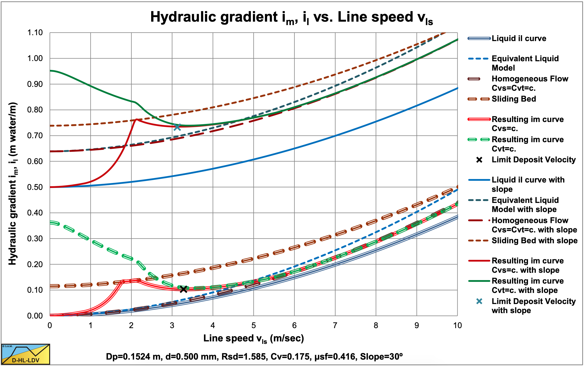
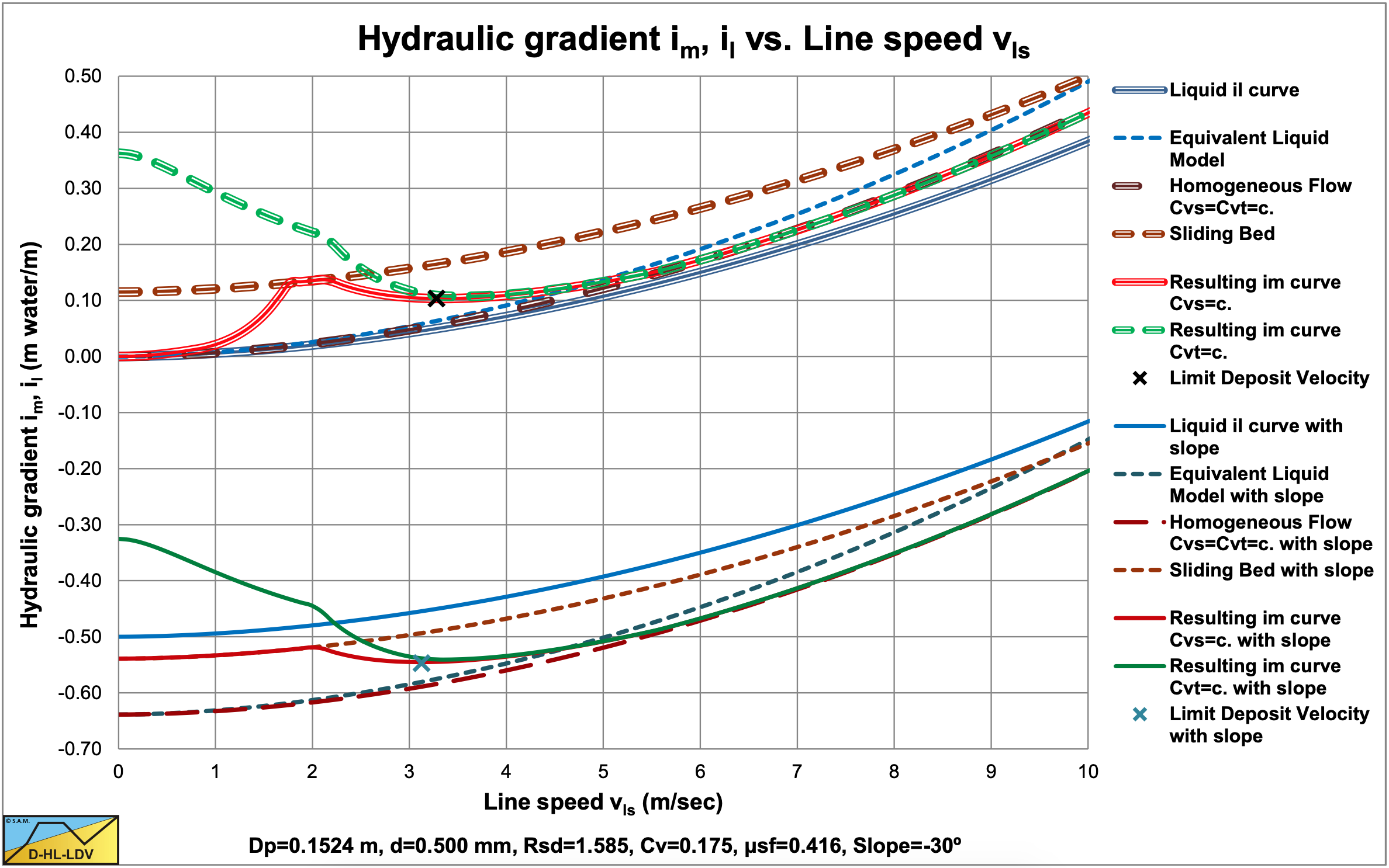
Figure 7.14-7 and Figure 7.14-8 show the hydraulic gradient in a horizontal pipe with D_p=0.1524 m and d=0.5 mm, an ascending pipe with slope 30^o and a descending pipe with slope -30^o. In a horizontal pipe, for constant spatial concentration, a sliding bed will occur. The ascending pipe does not show a sliding bed, in fact the resulting curve just touches the sliding bed curve at a higher line speed than the start of a sliding bed in a horizontal pipeline. The descending pipe show a sliding bed from zero line speed up to the line speed where the heterogeneous flow regime starts, which happens at a lower line speed than for the horizontal pipe.

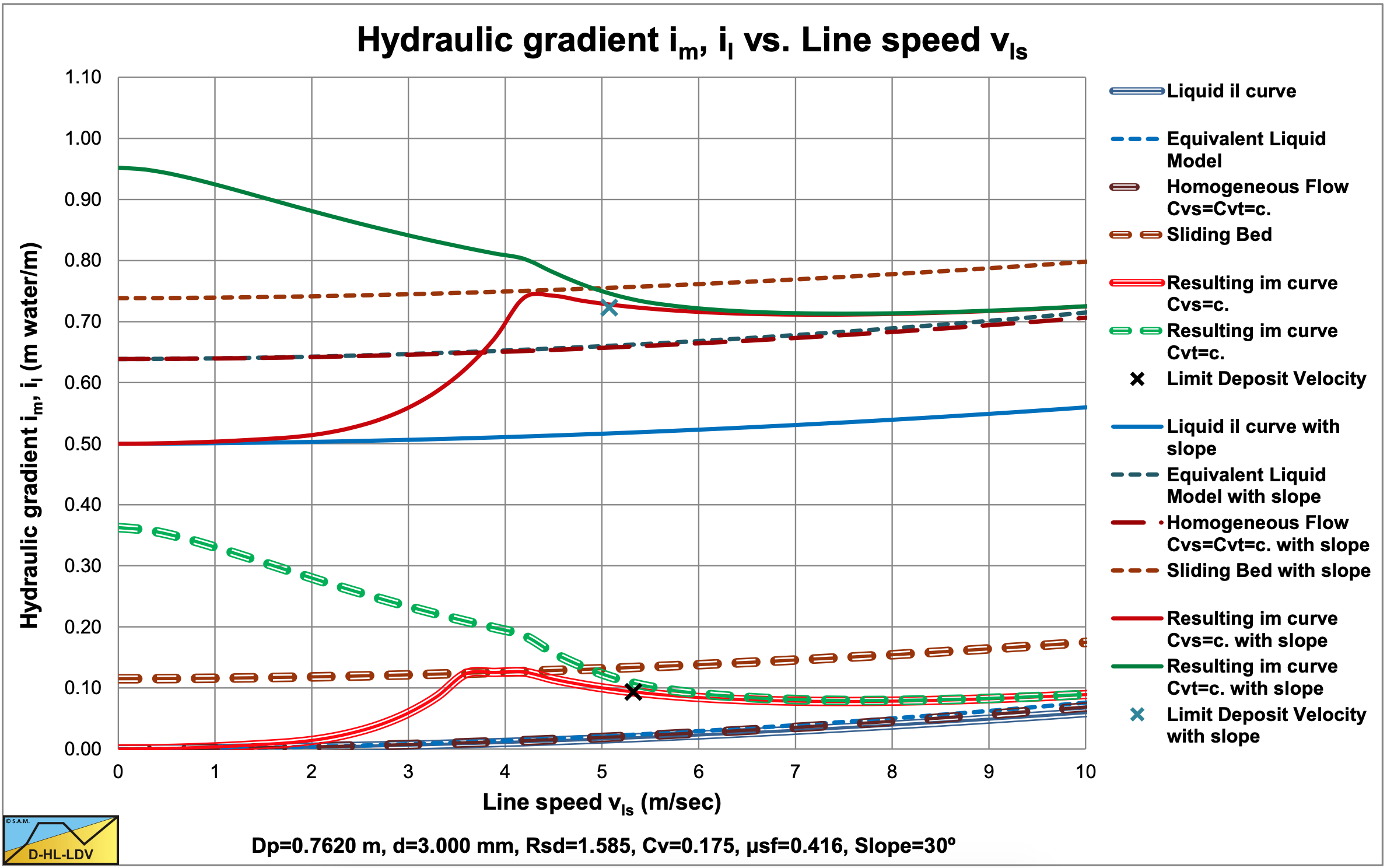
Figure 7.14-9 and Figure 7.14-10 show the same phenomena in a pipe with D_p=0.762 m. Here a d=3 mm particle is required to have a sliding bed. The figures also show a slight decrease of the Limit Deposit Velocity for the pipes with a slope.

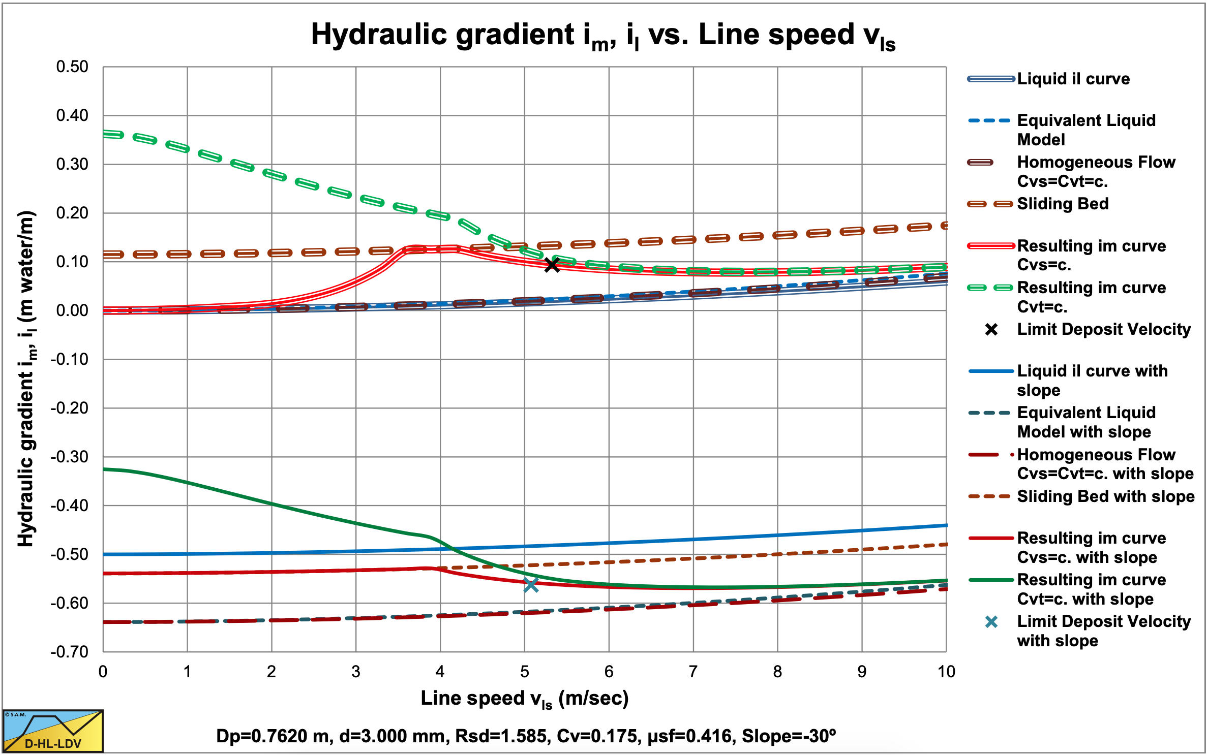
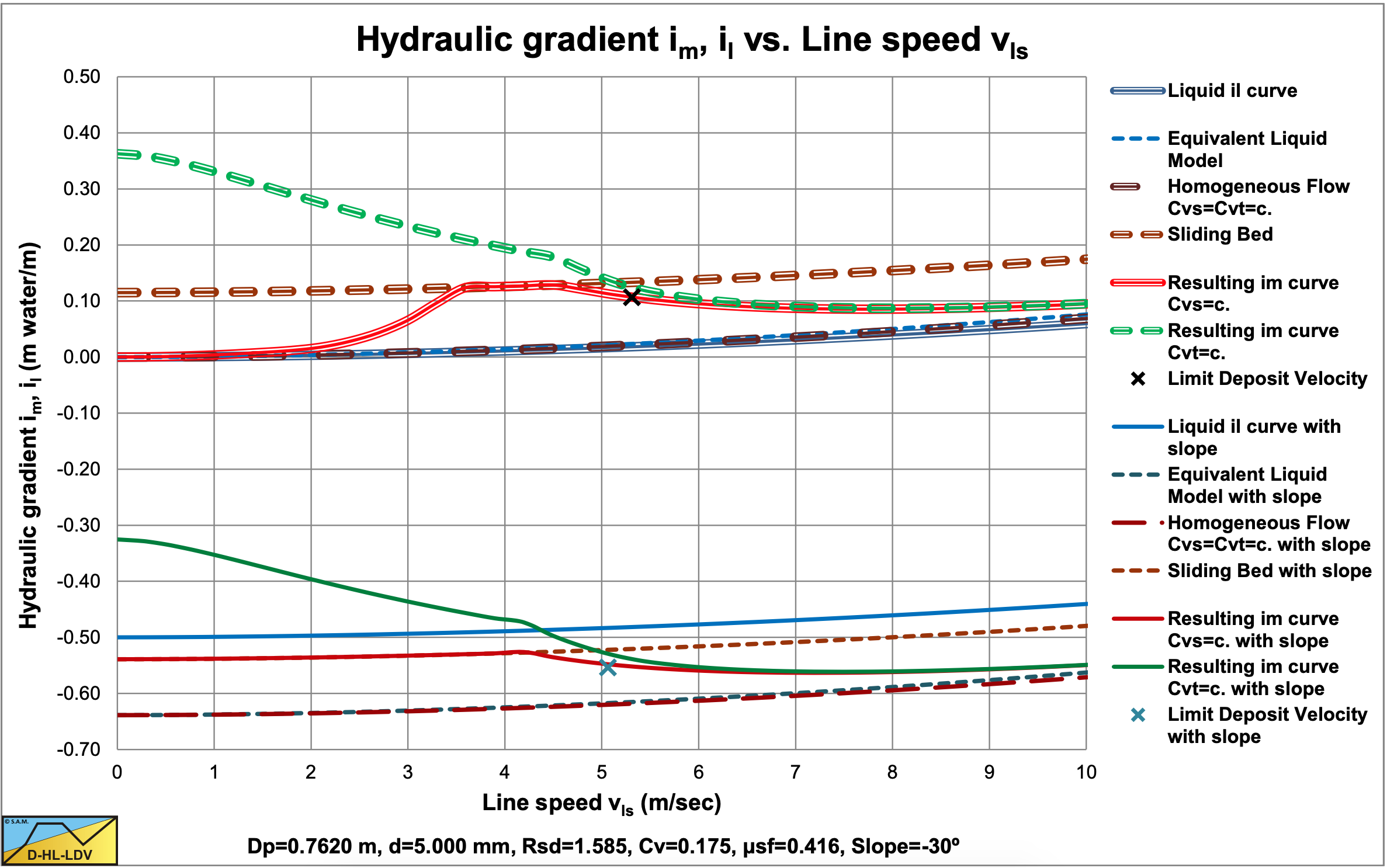
Figure 7.14-11 and Figure 7.14-12 show the same for a d=5 mm particle. Now the ascending pipeline also has a sliding bed, but it starts at a higher line speed and stops at a lower line speed, compared to the horizontal pipe. A sliding bed in an ascending pipe will encounter a higher bed shear stress and have a lower bed velocity, compared to a horizontal pipeline.

In order to find the correct hydraulic gradient curves for an inclined pipe, one first has to determine the hydraulic gradient curves for each flow regime individually. The resulting curve can be found by comparing flow regime curves.

1. If the sliding bed hydraulic gradient (SB) is smaller than the stationary (fixed) bed hydraulic gradient (FB), the sliding bed hydraulic gradient (SB) is chosen, otherwise the stationary bed hydraulic gradient. The resulting curve is named the FB-SB curve.
2. If the heterogeneous flow regime hydraulic gradient (He) is smaller than the FB-SB hydraulic gradient, the heterogeneous hydraulic gradient (He) is chosen, otherwise the FB-SB hydraulic gradient. The resulting curve is named the FB-SB-He curve. Depending on the parameters (particle and pipe diameter), it is possible that this curve does not contain a sliding bed regime.
3. If the homogeneous flow regime hydraulic gradient (Ho) is larger than the FB-SB-HE hydraulic gradient. The homogeneous hydraulic gradient (Ho) is chosen, otherwise the FB-SB-He hydraulic gradient. The resulting curve is named the FB-SB-He-Ho curve.

The hydraulic gradients of the inclined pipes are determined per meter of inclined pipe and not per meter of horizontal pipe.

Figure 7.14-7: The hydraulic gradient in an ascending pipeline, d=0.5 mm, D_p=0.1524 m.

Figure 7.14-8: The hydraulic gradient in a descending pipeline, d=0.5 mm, D_p=0.1524 m.

Figure 7.14-9: The hydraulic gradient in an ascending pipeline, d=3 mm, D_p=0.762 m.

Figure 7.14-10: The hydraulic gradient in a descending pipeline, d=3 mm, D_p=0.762 m.

Figure 7.14-11: The hydraulic gradient in an ascending pipeline, d=5 mm, D_p=0.762 m.

Figure 7.14-12: The hydraulic gradient in a descending pipeline, d=5 mm, D_p=0.762 m.

7.14.9 Nomenclature Inclined Pipes

A,Ap	Cross section pipe	m^2
A1	Cross section restricted area above the bed	m^2
A2	Cross section bed	m^2
c	Proportionality constant	-
Cvb	Bed volumetric concentration	-
Cvs	Spatial volumetric concentration	-
d	Particle diameter	m
Erhg	Relative excess hydraulic gradient without pipe inclination	-
Erhg,θ	Relative excess hydraulic gradient with pipe inclination	-
g	Gravitational constant (9.81)	m/s^2
il	Hydraulic gradient liquid without pipe inclination	-
il,θ	Hydraulic gradient liquid with pipe inclination	-
im	Hydraulic gradient mixture without pipe inclination	-
im,θ	Hydraulic gradient mixture with pipe inclination	-
L	Length of pipe	m
O1	Circumference restricted area above the bed in contact with pipe wall	m
O2	Circumference of bed with pipe wall	m
O12	Width of the top of the bed	m
p	Pressure in pipe	kPa
Rsd	Relative submerged density of solids	-
Shr	Settling velocity Hindered Relative without pipe inclination	-
Shr,θ	Settling velocity Hindered Relative with pipe inclination	-
Srs	Slip Ratio Squared without pipe inclination	-
Srs,θ	Slip Ratio Squared with pipe inclination	-
u*	Friction velocity	m/s
vls	Line speed	m/s
vt	Terminal settling velocity	m/s
vsl	Slip velocity solids	m/s
vls,ldv	Limit Deposity Velocity without pipe inclination	m/s
vls,ldv,θ	Limit Deposity Velocity with pipe inclination	m/s
Wb	Weight of the bed	ton
Wb,s	Submerged weight of the bed	ton
x	Distance in pipe length direction	m
αE	Homogeneous lubrication factor	-
β	Richardson & Zaki hindered settling power	-
δv	Thickness viscous sub-layer	m
ρb	Density of the bed including pore water	ton/m^3
ρs	Density of the solids	ton/m^3
ρl	Density of the liquid	ton/m^3
ρm	Mixture density	ton/m^3
\(\ \tau_{\mathrm{l}}\)	Shear stress between liquid and pipe wall	kPa
\(\ \tau_{ 12}\)	Shear stress on top of the bed	kPa
θ	Inclination angle (positive upwards, negative downwards)	^o
μsf	Sliding friction coefficient	-
κC	Concentration eccentricity factor	-