8.4: The Fixed or Stationary Bed Regime

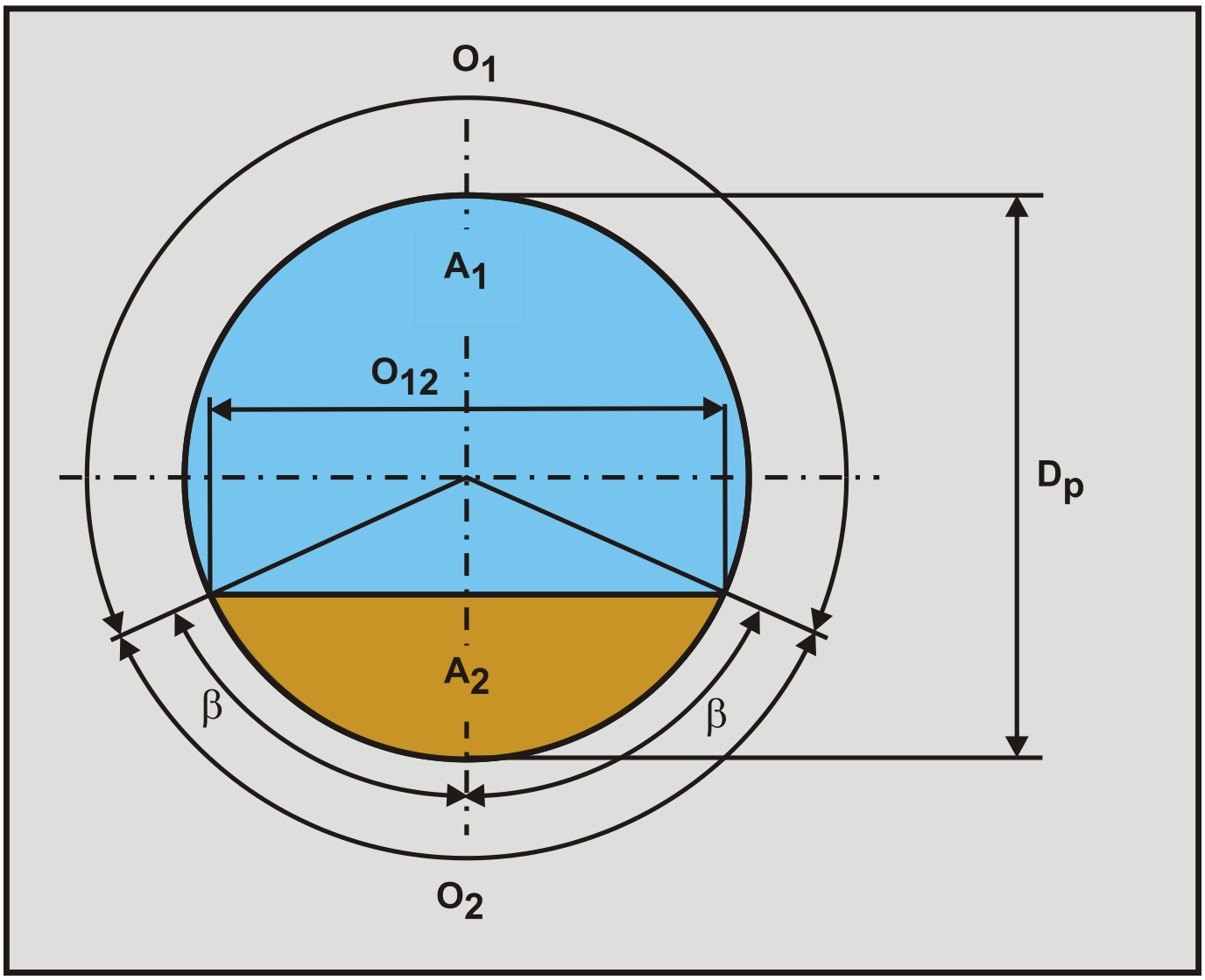
The fixed bed or stationary bed model is only required for determining the constant spatial volumetric concentration curves. For the constant delivered volumetric concentration curves, the sliding bed model forms the basis. The cross section of the pipe with a particle bed as defined in the Wilson et al. (1992) two layer model has been illustrated by Figure 8.4-1.

Figure 8.4-1: The definitions for fully stratified and heterogeneous flow.

The geometry is defined by the following equations. The length of the liquid in contact with the whole pipe wall, in a cross-section, if there is no bed is:

\[\ \mathrm{O}_{\mathrm{p}}=\pi \cdot \mathrm{D}_{\mathrm{p}}\]

The length of the liquid or the suspension in contact, in a cross-section, with the pipe wall:

\[\ \mathrm{O}_{\mathrm{1}}=\mathrm{D}_{\mathrm{p}} \cdot(\pi-\boldsymbol{\beta})\]

The length of the fixed or sliding bed in contact with the wall, in a cross-section:

\[\ \mathrm{O}_{2}=\mathrm{D}_{\mathrm{p}} \cdot \boldsymbol{\beta}\]

The top surface length of the fixed or sliding bed, in a cross-section:

\[\ \mathrm{O}_{12}=\mathrm{D}_{\mathrm{p}} \cdot \sin (\beta)\]

The cross sectional area A_p of the pipe is:

\[\ \mathrm{A_{p}=\frac{\pi}{4} \cdot D_{p}^{2}}\]

The cross sectional area A₂ of the fixed or sliding bed is:

\[\ \mathrm{A}_{2}=\mathrm{A}_{\mathrm{p}} \cdot \frac{\mathrm{C}_{\mathrm{v s}}}{\mathrm{C}_{\mathrm{vs}}}=\frac{\pi}{4} \cdot \mathrm{D}_{\mathrm{p}}^{2} \cdot \frac{(\beta-\sin (\beta) \cdot \cos (\beta))}{\pi}\]

The cross sectional area A₁ above the bed, where the liquid or the suspension is flowing, also named the restricted area, is:

\[\ \mathrm{A}_{1}=\mathrm{A}_{\mathrm{p}}-\mathrm{A}_{2}\]

The hydraulic diameter D_H,1 as function of the bed height, is equal to four times the cross sectional area divided by the wetted perimeter:

\[\ \mathrm{D}_{\mathrm{H}, \mathrm{1}}=\frac{\mathrm{4} \cdot \mathrm{A}_{1}}{\mathrm{O}_{\mathrm{1}}+\mathrm{O}_{12}} \quad\text{ or simplified: }\quad \mathrm{D}_{\mathrm{H}, \mathrm{1}}=\sqrt{\frac{4 \cdot \mathrm{A}_{1}}{\pi}}\]

The volume balance gives a relation between the line speed v_ls, the velocity in the restricted area above the bed v₁ and the velocity of the bed v₂.

\[\ \mathrm{v}_{\mathrm{l} \mathrm{s}} \cdot \mathrm{A}_{\mathrm{p}}=\mathrm{v}_{\mathrm{1}} \cdot \mathrm{A}_{\mathrm{1}}+\mathrm{v}_{\mathrm{2}} \cdot \mathrm{A}_{\mathrm{2}}\]

Thus the velocity in the restricted area above the bed is:

\[\ \mathrm{v}_{1}=\frac{\mathrm{v}_{\mathrm{l s}} \cdot \mathrm{A}_{\mathrm{p}}-\mathrm{v}_{2} \cdot \mathrm{A}_{2}}{\mathrm{A}_{1}}\]

And the velocity of the bed is (in the case of a fixed bed this is zero):

\[\ \mathrm{v}_{2}=\frac{\mathrm{v}_{\mathrm{l s}} \cdot \mathrm{A}_{\mathrm{p}}-\mathrm{v}_{\mathrm{1}} \cdot \mathrm{A}_{\mathrm{1}}}{\mathrm{A}_{2}}\]

8.4.1 The Shear Stresses Involved

In order to determine the forces involved, first the shear stresses involved have to be determined. Over the whole range of Reynolds numbers above 2320 the Swamee Jain equation gives a good approximation for the Darcy- Weisbach friction coefficient. For the flow in the restricted area above the bed, the shear stress between the liquid and the pipe wall is:

\[\ \tau_{1,\mathrm{l}}=\frac{\lambda_{1}}{4} \cdot \frac{1}{2} \cdot \rho_{\mathrm{l}} \cdot v_{1}^{2} \quad\text{ with: }\quad \lambda_{1}=\frac{1.325}{\left(\ln \left(\frac{0.27 \cdot \varepsilon}{\mathrm{D}_{\mathrm{H}, 1}}+\frac{5.75}{\mathrm{R} \mathrm{e}^{0.9}}\right)\right)^{2}} \quad\text{ and }\quad \operatorname{Re}=\frac{\mathrm{v}_{1} \cdot \mathrm{D}_{\mathrm{H}, 1}}{v_{\mathrm{l}}}\]

For the flow in the restricted area, the shear stress between the liquid and the bed for small values of v₁, when sheet flow is not occurring, is:

\[\ \tau_{12,\mathrm{l}}=\frac{\lambda_{12}}{4} \cdot \frac{1}{2} \cdot \rho_{\mathrm{l}} \cdot \mathrm{v_{l}}^{2} \quad\text{ with: }\quad \lambda_{12}=\frac{\alpha \cdot 1.325}{\left(\ln \left(\frac{0.27 \cdot \mathrm{d}}{\mathrm{D}_{\mathrm{H}, 1}}+\frac{5.75}{\mathrm{Re}^{0.9}}\right)\right)^{2}} \quad\text{ and }\quad \mathrm{Re}=\frac{\mathrm{v}_{1} \cdot \mathrm{D}_{\mathrm{H}, 1}}{v_{\mathrm{l}}}\]

For larger values of values of v₁, when sheet flow does occur, the following equation has to be applied:

\[\ \begin{array}{left} \tau_{12,\mathrm{l}}&=\frac{\lambda_{12}}{4} \cdot \frac{1}{2} \cdot \rho_{\mathrm{l}} \cdot \mathrm{v}_{1}^{2} \quad \text { with: } \\ \lambda_{12}&= 0.83 \cdot \lambda_{1}+0.37 \cdot\left(\frac{\mathrm{v}_{1}}{\sqrt{2 \cdot \mathrm{g} \cdot \mathrm{D}_{\mathrm{H}, 1} \cdot \mathrm{R}_{\mathrm{sd}}}}\right)^{2.73} \cdot\left(\frac{\rho_{\mathrm{s}} \cdot \frac{\pi}{6} \cdot \mathrm{d}^{3}}{\rho_{\mathrm{l}} \cdot 1^{3}}\right)^{0.094} \\ &= 0.83 \cdot \lambda_{1}+0.37 \cdot \mathrm{Fr}_{\mathrm{DC}}^{2.73} \cdot\left(\frac{\mathrm{m}_{\mathrm{p}}}{\rho_{\mathrm{l}}}\right)^{0.094} \end{array}\]

Miedema & Matousek (2014) derived the above equation, except for the particle mass term, which is added by Miedema & Ramsdell (2014). This last term increases the correlation coefficient of the curve fit of experimental data from 0.86 (without this term) to 0.91 (including this term). Reason for adding this last term is, that in sheet flow energy losses are not only determined by the submerged weight of the particles, but also by the mass of the particles. The use of equations (7.3-18)(8.4-13) and (7.3-57)(8.4-14) is simple, if equation (7.3-57)(8.4-14)>(7.3-18)(8.4-13), equation (7.3-57)(8.4-14) is used and sheet flow is assumed, otherwise equation (7.3-18)(8.4-13) is used and a flat bed with maybe individual particles moving is assumed.

8.4.2 The Forces Involved

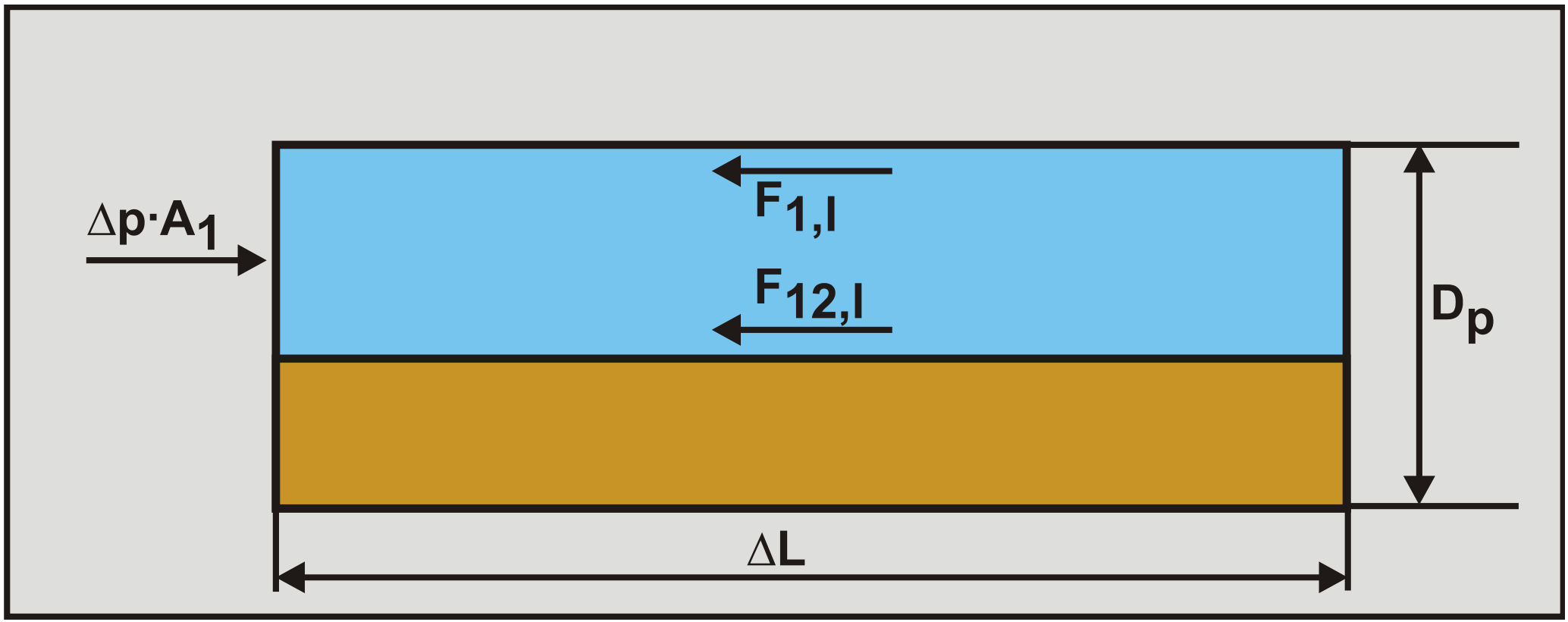
First the equilibrium of the forces on the liquid above the bed is determined. This is necessary to find the correct hydraulic gradient.

The resisting shear force on the pipe wall O₁ above the bed is:

\[\ \mathrm{F}_{1,\mathrm{l}}=\tau_{1,\mathrm{l}} \cdot \mathrm{O}_{1} \cdot \Delta \mathrm{L}\]

The resisting shear force on the bed surface O₁₂ is:

\[\ \mathrm{F}_{12,\mathrm{l}}=\tau_{12,\mathrm{l}} \cdot \mathrm{O}_{12} \cdot \Delta \mathrm{L}\]

The pressure Δp on the liquid above the bed is:

\[\ \Delta \mathrm{p}=\Delta \mathrm{p}_{2}=\Delta \mathrm{p}_{1}=\frac{\tau_{1,\mathrm{l}} \cdot \mathrm{O}_{1} \cdot \Delta \mathrm{L}+\tau_{12,\mathrm{l}} \cdot \mathrm{O}_{12} \cdot \Delta \mathrm{L}}{\mathrm{A}_{1}}=\frac{\mathrm{F}_{1,1}+\mathrm{F}_{12, \mathrm{l}}}{\mathrm{A}_{1}}\]

Figure 8.4-2: The forces on the liquid above the bed.

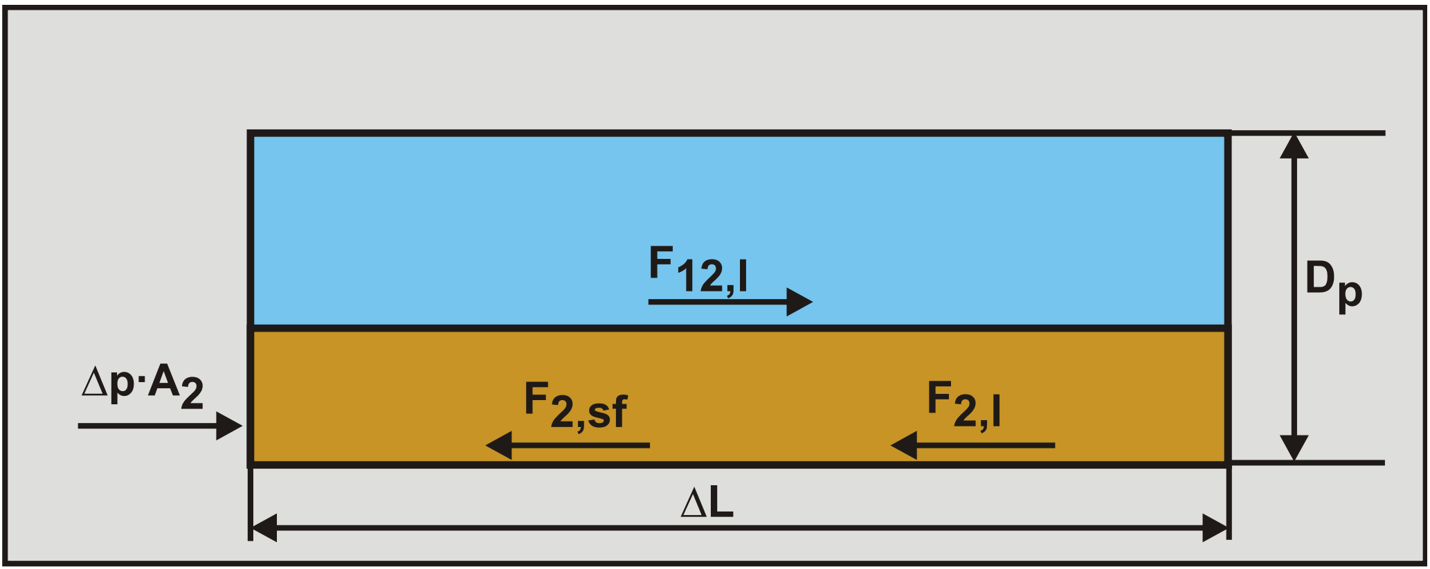
The force equilibrium on the liquid above the bed is shown in Figure 8.4-2. Secondly the equilibrium of forces on the bed is determined as is shown in Figure 8.4-3.

Figure 8.4-3: The forces on the bed.

The driving shear force on the bed surface is:

\[\ \mathrm{F}_{12,\mathrm{l}}=\tau_{12,\mathrm{l}} \cdot \mathrm{O}_{12} \cdot \Delta \mathrm{L}\]

The driving force resulting from the pressure Δp on the bed is:

\[\ \mathrm{F}_{2, \mathrm{p r}}=\Delta \mathrm{p} \cdot \mathrm{A}_{2}\]

The resisting force between the bed and the pipe wall due to sliding friction is:

\[\ \mathrm{F}_{2, \mathrm{sf}}=\tau_{2, \mathrm{sf}} \cdot \mathrm{O}_{2} \cdot \Delta \mathrm{L}\]

The resisting shear force between the liquid in the bed and the pipe wall is:

\[\ \mathrm{F}_{2,\mathrm{l}}=\tau_{2,\mathrm{l}} \cdot \mathrm{O}_{2} \cdot \mathrm{n} \cdot \Delta \mathrm{L}\]

This shear force is multiplied by the porosity n, in order to correct for the fact that the bed consists of a combination of particles and water. There is an equilibrium of forces when:

\[\ \mathrm{F}_{12,\mathrm{l}}+\mathrm{F}_{2, \mathrm{p r}}=\mathrm{F}_{2, \mathrm{s f}}+\mathrm{F}_{2, \mathrm{l}}\]

Below the Limit of Stationary Deposit Velocity, the bed is not sliding and the force F_2,l equals zero. Equation (7.3-24)(8.4-17) is used to determine the pressure losses with a stationary bed. Since the problem is implicit with respect to the velocities v₁ and v₂, it has to be solved with an iteration process.

The mixture pressure is now:

\[\ \Delta \mathrm{p}_{\mathrm{m}}=\frac{\lambda_{1} \cdot \mathrm{O}_{1}+\lambda_{12} \cdot \mathrm{O}_{12}}{\mathrm{4} \cdot\left(\mathrm{1}-\mathrm{C}_{\mathrm{v r}}\right) \cdot \mathrm{A}_{\mathrm{p}}} \cdot \frac{\mathrm{1}}{2} \cdot \rho_{\mathrm{l}} \cdot \mathrm{v}_{\mathrm{1}}^{2} \cdot \Delta \mathrm{L} \quad\text{ with: }\quad \mathrm{C}_{\mathrm{v r}}=\frac{\mathrm{C}_{\mathrm{v s}}}{\mathrm{C}_{\mathrm{v b}}}\]

8.4.3 Pressure, Hydraulic Gradient & Relative Solids Effect

The excess pressure and excess hydraulic gradient can be written as:

\[\ \begin{array}{left}\Delta \mathrm{p}_{\mathrm{m}}-\Delta \mathrm{p}_{\mathrm{l}}=\left(\left(\lambda_{1} \cdot \mathrm{O}_{1}+\lambda_{12} \cdot \mathrm{O}_{12}\right) \cdot\left(\frac{\mathrm{1}}{\mathrm{1}-\mathrm{C}_{\mathrm{v r}}}\right)^{\mathrm{3}}-\lambda_{\mathrm{l}} \cdot \mathrm{O}_{\mathrm{p}}\right) \cdot \frac{\mathrm{1}}{2} \cdot \rho_{\mathrm{l}} \cdot \mathrm{v}_{\mathrm{l} \mathrm{s}}^{2} \cdot \frac{\Delta \mathrm{L}}{4 \cdot \mathrm{A}_{\mathrm{p}}}\\
\text{and}\\
\mathrm{i}_{\mathrm{m}}-\mathrm{i}_{\mathrm{l}}=\left(\left(\lambda_{1} \cdot \mathrm{O}_{1}+\lambda_{12} \cdot \mathrm{O}_{12}\right) \cdot\left(\frac{\mathrm{1}}{\mathrm{1}-\mathrm{C}_{\mathrm{v} \mathrm{r}}}\right)^{\mathrm{3}}-\lambda_{\mathrm{l}} \cdot \mathrm{O}_{\mathrm{p}}\right) \cdot \frac{\mathrm{v}_{\mathrm{l s}}^{2}}{\mathrm{8} \cdot \mathrm{g} \cdot \mathrm{A}_{\mathrm{p}}}\end{array}\]

In terms of the relative excess hydraulic gradient or relative solids effect this can be written as:

\[\ \mathrm{E}_{\mathrm{rhg}}=\frac{\mathrm{i}_{\mathrm{m}}-\mathrm{i}_{\mathrm{l}}}{\mathrm{R}_{\mathrm{s d}} \cdot \mathrm{C}_{\mathrm{v s}}}=\left(\left(\lambda_{1} \cdot \mathrm{O}_{\mathrm{1}}+\lambda_{12} \cdot \mathrm{O}_{12}\right) \cdot\left(\frac{\mathrm{1}}{\mathrm{1 - C}_{\mathrm{v r}}}\right)^{\mathrm{3}}-\lambda_{\mathrm{l}} \cdot \mathrm{O}_{\mathrm{p}}\right) \cdot \frac{\mathrm{v}_{\mathrm{l s}}^{2}}{\mathrm{8 \cdot g \cdot A _ { \mathrm { p } }} \cdot \mathrm{R}_{\mathrm{s d}} \cdot \mathrm{C}_{\mathrm{v s}}}\]

For practical purposes, the stationary/fixed bed regime is not very usefull and can be replaced by the sliding bed regime, also for very low line speeds. In all the DHLLDV Framework graphs however it has been taken into account for the constant spatial volumetric concentration curves, showing the LSDV as the intersection of the fixed bed curve and the sliding bed curve.