
1.7: Deflection of Beams- Geometric Methods
- Page ID
- 17613

Deflection of Beams: Geometric Methods
The serviceability requirements limit the maximum deflection that is allowed in a structural element subjected to external loading. Excessive deflection may result in the discomfort of the occupancy of a given structure and can also mar its aesthetics. Most codes and standards provide the maximum allowable deflection for dead loads and superimposed live loads. To ensure that the possible maximum deflection that could occur under a given loading is within acceptable value, the structural component is usually analyzed for deflection, and the determined maximum deflection value is compared with the specified values in the codes and standards of practice.
There are several methods of determining the deflection of a beam or frame. The choice of a particular method is dependent on the nature of the loading and the type of problem being solved. Some of the methods used in this chapter include the method of double integration, the method of singularity function, the moment-area method, the unit-load method, the virtual work method, and the energy methods.
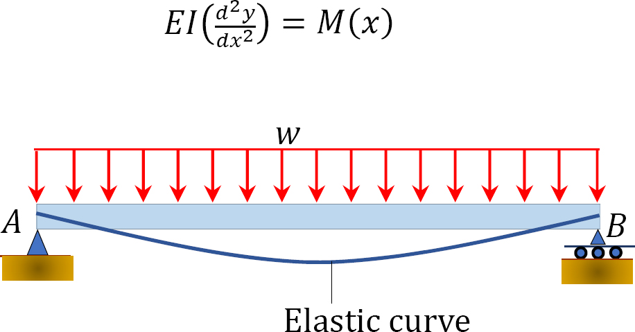
7.2 Derivation of the Equation of the Elastic Curve of a Beam
The elastic curve of a beam is the axis of a deflected beam, as indicated in Figure 7.1a.

To derive the equation of the elastic curve of a beam, first derive the equation of bending.
Consider the portion cdef of the beam shown in Figure 7.1a, subjected to pure moment, M, for the derivation of the equation of bending. Due to the applied moment M, the fibers above the neutral axis of the beam will elongate, while those below the neutral axis will shorten. Let O be the center and R be the radius of the beam’s curvature, and let ij be the axis of the curved beam. The beam subtends an angle θ at O. And let σ be the longitudinal stress in a filament gℎ at a distance y from the neutral axis.
From geometry, the length of the neutral axis of the beam ij and that of the filament gℎ, located at a distance y from the neutral axis of the beam, can be computed as follows:

The strain ε in the filament can be computed as follows:

For a linear elastic material, in which Hooke’s law applies, equation 7.1 can be written as follows:


The force on the entire cross-section of the beam then becomes:

From static equilibrium consideration, the external moment M in the beam is balanced by the moments about the neutral axis of the internal forces developed at a section of the beam. Thus,

Substituting 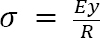 from equation 7.2 into equation 7.5 suggests the following:

Putting I = ∫ y2δA into equation 7.6 suggests the following:

where
I = the moment of inertia or the second moment of area of the section.
Combining equations 7.2 and 7.7 suggests the following:

The equation of the elastic curve of a beam can be found using the following methods.
From differential calculus, the curvature at any point along a curve can be expressed as follows:
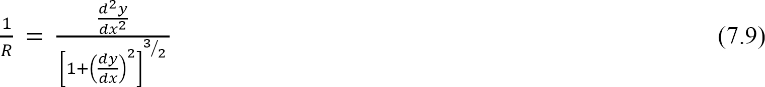
where
 are the first and second derivative of the function representing the curve in terms of the Cartesian coordinates x and y.
 which represents the slope of the curve at any point of the deformed beam, will also be small. Since
  is negligibly insignificant, equation 7.9 could be simplified as follows:
Combining equations 7.2 and 7.10 suggests the following:

Rearranging equation 7.11 yields the following:

Equation 7.12 is referred to as the differential equation of the elastic curve of a beam.
7.3 Deflection by Method of Double Integration
Deflection by double integration is also referred to as deflection by the method of direct or constant integration. This method entails obtaining the deflection of a beam by integrating the differential equation of the elastic curve of a beam twice and using boundary conditions to determine the constants of integration. The first integration yields the slope, and the second integration gives the deflection. This method is best when there is a continuity in the applied loading.
Example 7.1
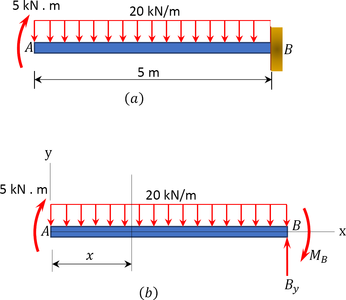
A cantilever beam is subjected to a combination of loading, as shown in Figure 7.2a. Using the method of double integration, determine the slope and the deflection at the free end.
Solution
Equation for bending moment. Passing a section at a distance x from the free-end of the beam, as shown in the free-body diagram in Figure 7.2b, and considering the moment to the right of the section suggests the following:

Substituting M into equation 7.12 suggests the following:

Equation for slope. Integrating with respect to x suggests the following:

Observe that at the fixed end where 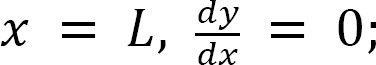 this is referred to as the boundary condition. Applying these boundary conditions to equation 3 suggests the following:
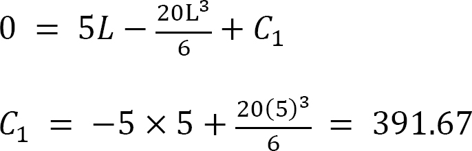
To obtain the following equation of slope, substitute the computed value of C1 into equation 3 follows:

Equation for deflection. Integrating equation 4 suggests the following:

At the fixed end x = L, y = 0. Applying these boundary conditions to equation 5 suggests the following:

To obtain the following equation of elastic curve, substitute the computed value of C2 into equation 5, as follows:

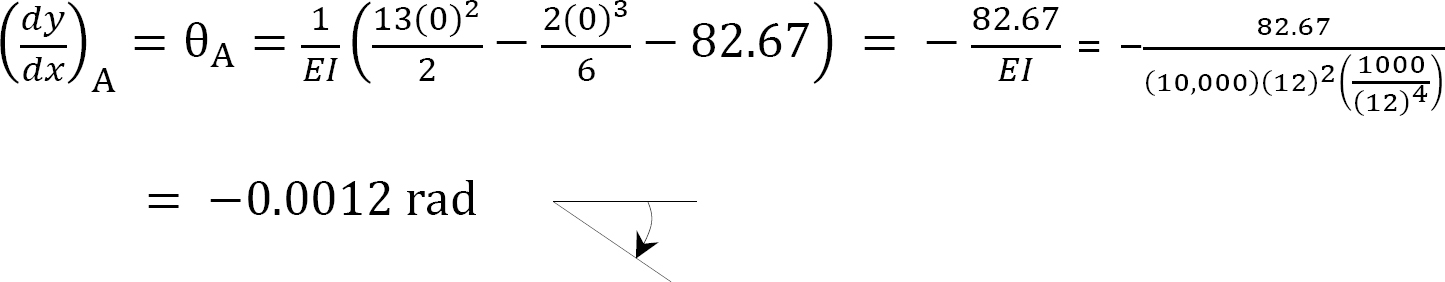
The slope at the free end, i.e.,  at x = 0

The deflection at the free end, i.e., y at x = 0

Example 7.2
A simply supported beam AB carries a uniformly distributed load of 2 kips/ft over its length and a concentrated load of 10 kips in the middle of its span, as shown in Figure 7.3a. Using the method of double integration, determine the slope at support A and the deflection at a midpoint C of the beam.

Solution
Support reactions.
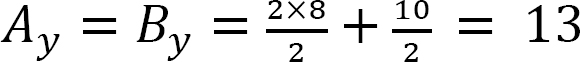 kips by symmetry
Substituting for M into equation 7.12 suggests the following:

Equation for slope. Integrating equation 2 with respect to x suggests the following:

The constant of integration C1 is evaluated by considering the boundary condition.
Applying the afore-stated boundary conditions to equation 3 suggests the following:
Bringing the computed value of C1 back into equation 3 suggests the following:

Equation for deflection. Integrating equation 4 suggests the following:

The constant of integration C2 is evaluated by considering the boundary condition.
At x = 0, y = 0
0 = 0 – 0 – 0 + C2
C2 = 0
Carrying the computed value of C2 back into equation 5 suggests the following equation of elastic curve:

The slope at 
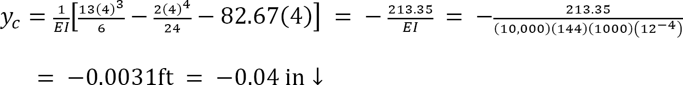
Deflection at midpoint 
Example 7.3
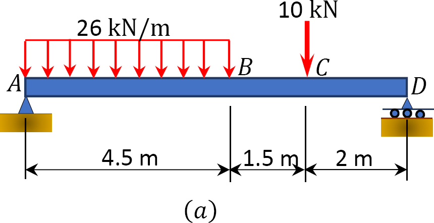
A beam carries a distributed load that varies from zero at support A to 50 kN/m at its overhanging end, as shown in Figure 7.4a. Write the equation of the elastic curve for segment AB of the beam, determine the slope at support A, and determine the deflection at a point of the beam located 3 m from support A.

Solution
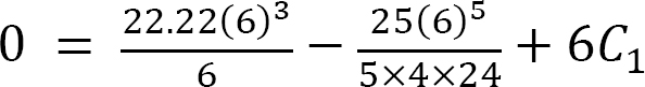
Support reactions. To determine the reactions of the beam, apply the equations of equilibrium, as follows:


Substituting for M into equation 7.12 suggests the following:

Equation for slope. Integrating equation 2 with respect to x suggests the following:

Equation for deflection. Integrating equation 3 suggests the equation of deflection, as follows:

To evaluate the constants of integrations, apply the following boundary conditions to equation 4:
At x = 0, y = 0
0 = 0 – 0 + 0 + C2
C2 = 0
At x = 6 m, y = 0
C1 = –65.82
Equation of elastic curve.
The equation of elastic curve can now be determined by substituting C1 and C2 into equation 4.
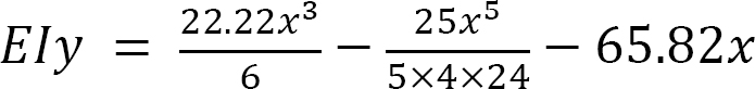
To obtain the equations of slope and deflection, substitute the computed value of C1 and C2 back into equations 3 and 4:
Equation of slope.

Equation of deflection.
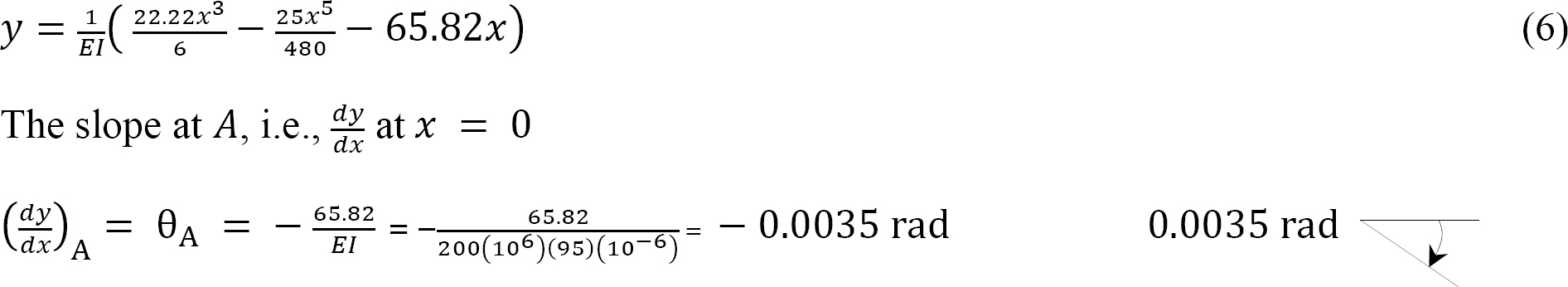
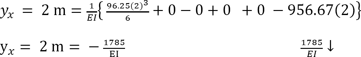
Deflection at x = 3 m from support A.

7.4 Deflection by Method of Singularity Function
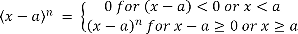
In cases where a beam is subjected to a combination of distributed loads, concentrated loads, and moments, using the method of double integration to determine the deflections of such beams is really involving, since various segments of the beam are represented by several moment functions, and much computational efforts are required to find the constants of integration. Using the method of singularity function in such cases to determine deflections is comparatively easier and relatively quick. This method of analysis was first introduced by Macaulay in 1919, and it entails the use of one equation that contains a singularity or half-range function to describe the entire beam deflection curve. A singularity or half-range function is defined as follows:
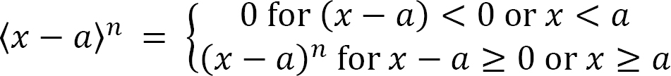
where
x = coordinate position of a point along the beam.
a = any location along the beam where discontinuity due to bending occurs.
n = the exponential values of the functions; this must always be greater than or equal to zero for the functions to be valid.
The above outlined definition implies that the quantity (x – a) equals zero or vanishes if it is negative, but it is equal to (x – a) if it is positive.
Procedure for Analysis by Singularity Function Method
•Sketch the free-body diagram of the beam and establish the x and y coordinates.
•Calculate the support reactions and write the moment equation as a function of the x coordinate. The sign convention for the moment is the same as in section 4.3.
•Substitute the moment expression into the equation of the elastic curve and integrate once to obtain the slope. Integrate again to obtain the deflection in the beam.
•Using the boundary conditions, determine the integration constants and substitute them into the equations obtained in step 3 to obtain the slope and the deflection of the beam. A positive slope is counterclockwise and a negative slope is clockwise, while a positive deflection is upward and a negative deflection is downward.
•When computing the slope or deflection at any point on the beam, discard the quantity (x – a) from the equation for slope or deflection if it is negative. If (x – a) is positive, it remains in the equation.
Example 7.4
A simply supported beam is subjected to the combined loading shown in Figure 7.5a. Using the method of singularity function, determine the slope at support A and the deflection at B.

Solution
Support reactions. To determine the reaction at support A of the beam, apply the equations of equilibrium, as follows:
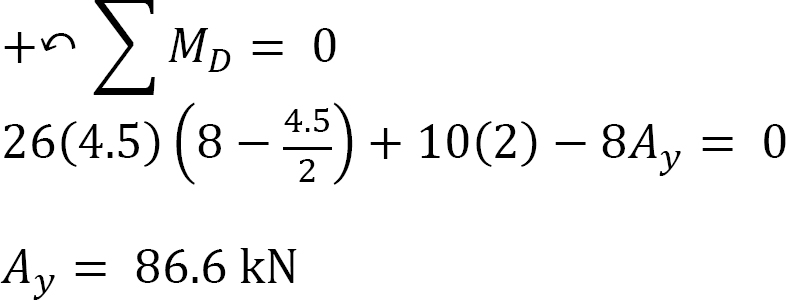

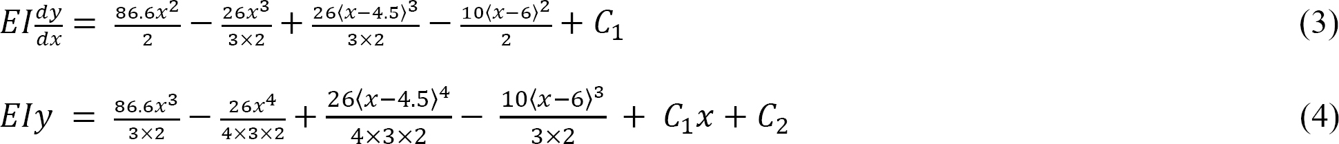
Equation of the elastic curve. Substituting for M(x) from equation 1 into equation 7.12 suggests the following:

Integrating equation 2 twice suggests the following:
Boundary conditions and computation of constants of integration. Applying the boundary conditions [x = 0, y = 0] to equation 4 and noting that each bracket contains a negative quantity and, thus, is equal zero by the singularity definition suggests that C2 = 0.
0 = 0 – 0 + 0 – 0 + C2
C2 = 0
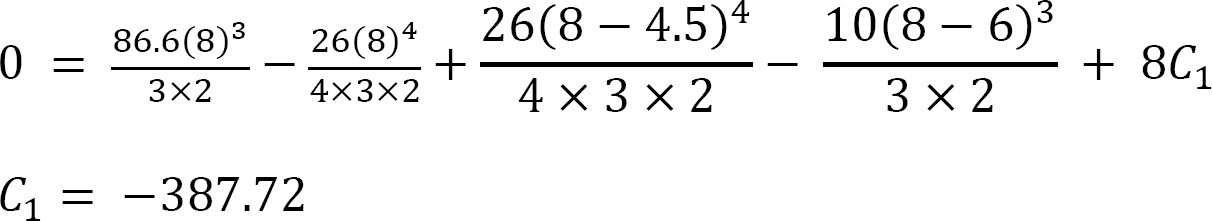
Again, applying the boundary conditions [x = 8, y = 0] to equation 4 and noting that each bracket contains a positive quantity suggests that the value of the constant C1 is as follows:
Substituting the values for C1 and C2 into equation 4 suggets that the expression for the elastic curve of the beam is as follows:

Similarly, substituting the values for C1 into equation 3 suggests the expression for the slope is as follows:

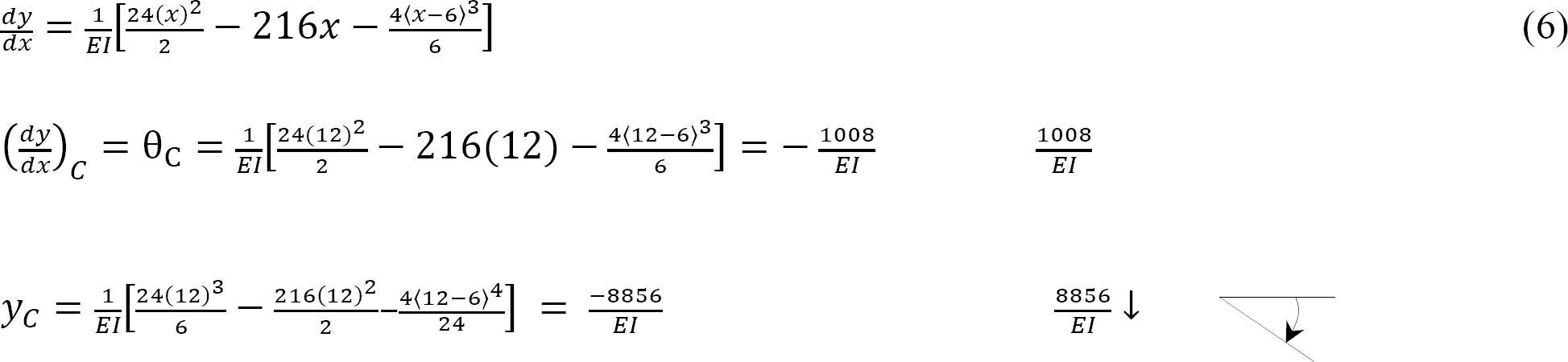
The slope at 

The deflection at x = 4.5 m from support A
Example 7.5
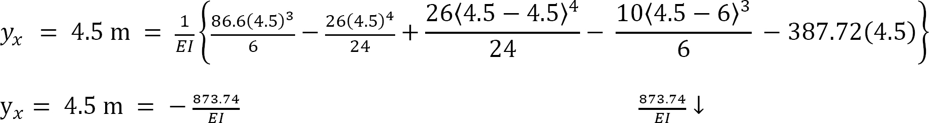
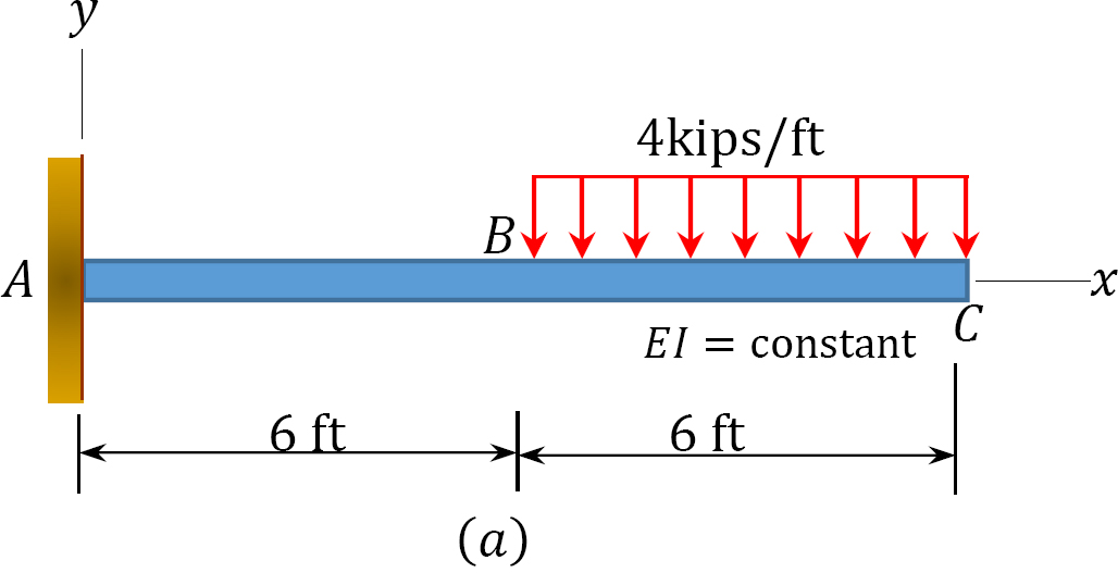
A cantilever beam is loaded with a uniformly distributed load of 4 kips/ft, as shown in Figure 7.6a. Using the method of singularity function, determine the equation of the elastic curve of the beam, the slope at the free end, and the deflection at the free end.
Solution
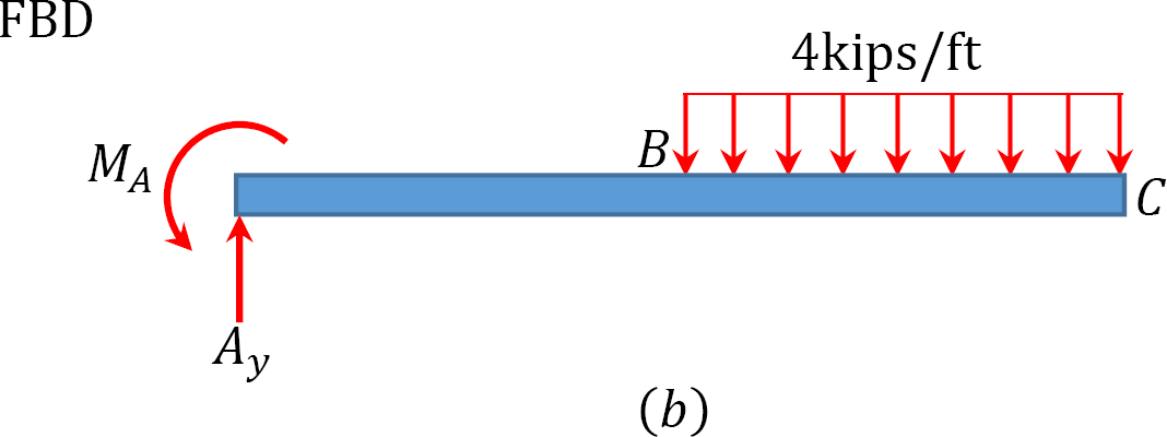
Support reactions. To determine the reaction at support A of the beam, apply the equation of equilibrium, as follows:


Equation of the elastic curve. Substituting for M(x) from equation 1 into equation 7.12 suggests the following:

Integrating equation 2 twice suggests the following:

Boundary conditions and computation of constants of integration. Applying the boundary conditions 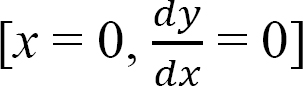 to equation 3 and noting that the term with a bracket contains a negative quantity and, thus, is equal to zero by the singularity function definition suggests that C1 = 0.

Applying the boundary conditions [x = 0, y = 0] to equation 4 and noting that the term with a bracket contains a negative quantity and, thus, is equal to zero by the singularity function definition suggests that C2 = 0.

To find the elastic curve of the beam, substitute the values for C1 and C2 into equation 4, as follows:

Similarly, to find the expression for the slope, substitute the values for C1 into equation 3, as follows:
Example 7.6
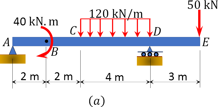
A beam with an overhang is subjected to a combined loading, as shown in Figure 7.7a. Using the method of the singularity function, determine the slope at support A and the deflection at B.

Solution
Support reactions. To determine the reaction at support A of the beam, apply the equations of equilibrium, as follows:


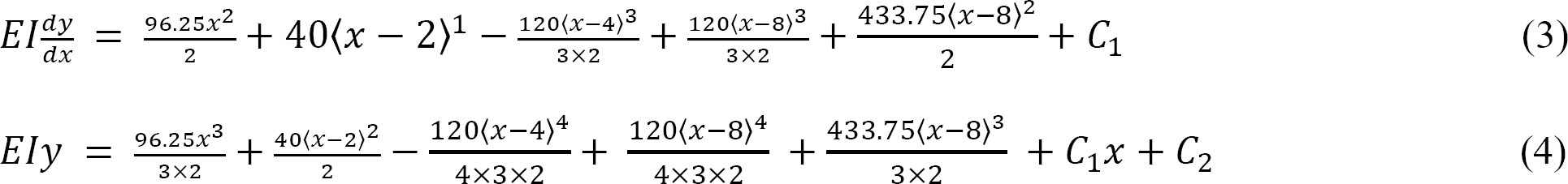
Equation of the elastic curve. Substituting for M(x) from equation 1 into equation 7.12 suggests the following:

Integrating equation 2 twice suggests the following:
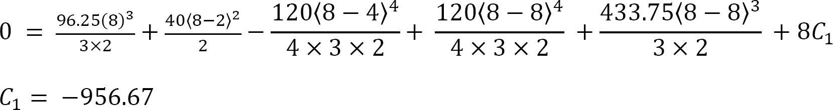
Boundary conditions and computation of constants of integration. Applying the boundary conditions [x = 0, y = 0] to equation 4 and noting that each bracket contains a negative quantity and, thus, is equal to zero by the singularity definition suggests that C2 = 0.
0 = 0 + 0 – 0 + 0 + 0 + 0 + C2
C2 = 0
Again, applying the boundary conditions [x = 8m, y = 0] to equation 4 and noting that each bracket contains a positive quantity suggests that the value of the constant C1 is as follows:
Substituting the values for C1 and C2 into equation 4 suggests that the expression for the elastic curve of the beam is as follows:

Similarly, substituting the values for C1 into equation 3 suggests that the expression for the slope is as follows:

The slope at 

The deflection at x = 2 m from support A
7.5 Deflection by Moment-Area Method
The moment-area method uses the area of moment divided by the flexural rigidity (M/EI) diagram of a beam to determine the deflection and slope along the beam. There are two theorems used in this method, which are derived below.
7.5.1 First Moment-Area Theorem
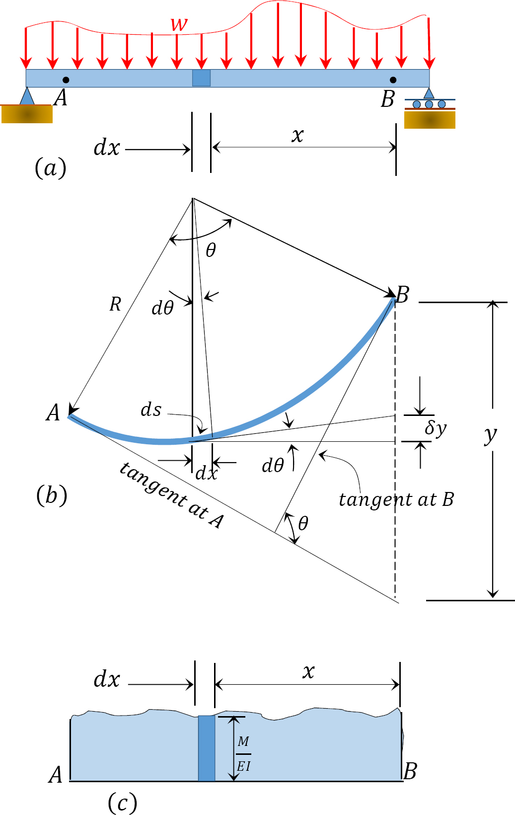
To derive the first moment-area theorem, consider a portion AB of an elastic curve of the deflected beam shown in Figure 7.8b. The beam has a radius of curvature R. Figure 7.8c represents the bending moment of this portion. According to geometry, the length of the arc ds, of the radius R, subtending an angle dθ, is equal to the product of the radius of curvature and the angle subtend. Therefore,

Rearranging equation 1 suggests the following:

Substituting equation 7.14 into equation 7.8 suggests the following:

Since ds is infinitesimal because of the small lateral deflection of the beam that is allowed in engineering, it can be replaced by its horizontal projection dx. Thus,

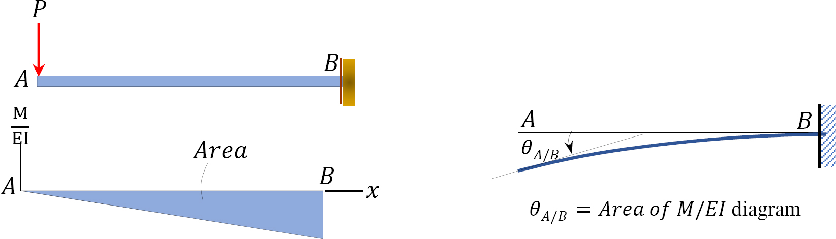
The angle θ between the tangents at A and B can thus be obtained by summing up the subtended angles by the infinitesimal length lying between these points. Thus,
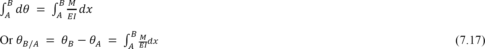
Equation 7.17 is referred to as the first moment-area theorem. The first moment-area theorem states that the total change in slope between A and B is equal to the area of the bending moment diagram between these two points divided by the flexural rigidity EI.
7.5.2 Second Moment-Area Theorem
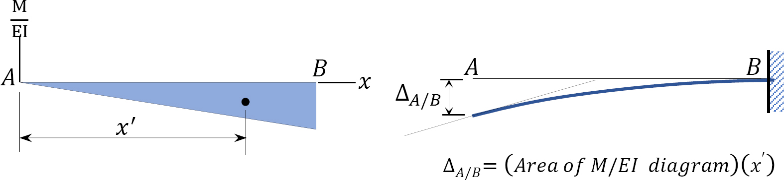
Referring again to Figure 7.8, it is required to determine the tangential deviation of point B with respect to point A, which is the vertical distance of point B from the tangent drawn to the elastic curve at point A. To do so, first calculate the contribution δ∆ of the element of length dL to the vertical distance. According to geometry,

Substituting dθ from equation 7.15 to equation 7.18 suggests the following:

Hence,

Equation 7.20 is referred to as the second moment area theorem. The second moment-area theorem states that the vertical distance of point B on an elastic curve from the tangent to the curve at point A is equal to the moment with respect to the vertical through B of the area of the bending moment diagram between A and B, divided by the flexural rigidity, EI.
7.5.3 Sign Conventions
The sign conventions for moment-area theorems are as follows:
(1)The tangential deviation of a point B, with respect to a tangent drawn at the elastic curve at a point A, is positive if B lies above the drawn tangent at A and negative if it lies below the tangent (see Figure 7.9).
(2)The slope at a point B, with respect to a tangent drawn at a point A in an elastic curve, is positive if the tangent drawn at B rotates in a counterclockwise direction with respect to the tangent at A and negative if it rotates in a clockwise direction (see Figure 7.9).

Procedure for Analysis by Moment-Area Method
•Sketch the free-body diagram of the beam.
•Draw the M/EI diagram of the beam. This will look like the conventional bending moment diagram of the beam if the beam is prismatic (i.e. of the same cross section for its entire length).
•To determine the slope at any point, find the angle between a tangent passing the point and a tangent passing through another point on the deflected curve, divide the M/EI diagram into simple geometric shapes, and then apply the first moment-area theorem. To determine the deflection or a tangential deviation of any point along the beam, apply the second moment-area theorem.
•In cases where the configuration of the M/EI diagram is such that it cannot be divided into simple shapes with known areas and centroids, it is preferable to draw the M/EI diagram by parts. This entails introducing a fixed support at any convenient point along the beam and drawing the M/EI diagram for each of the applied loads, including the support reactions, prior to the application of any of the theorems to determine what is required.
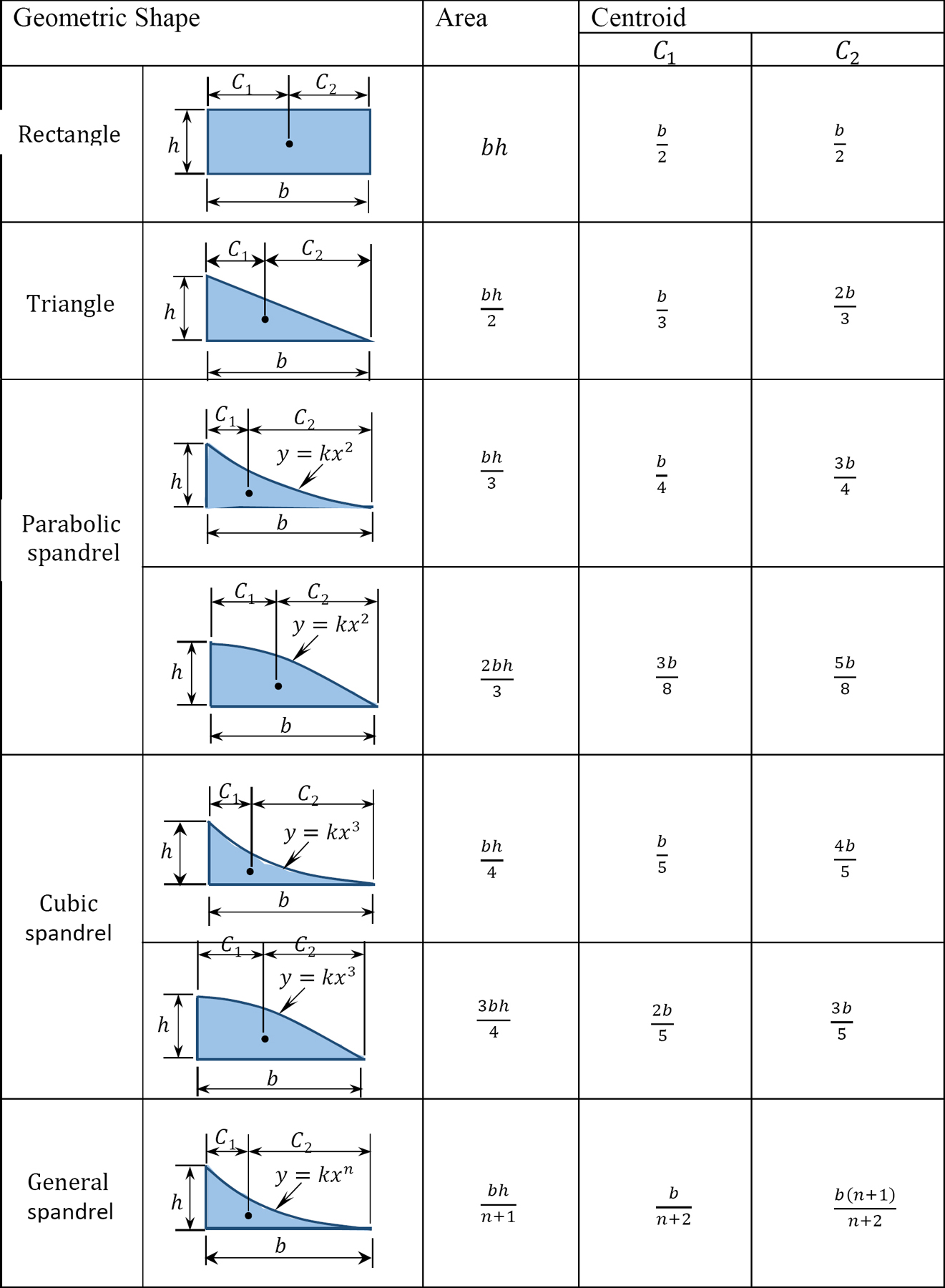
Table 7.1. Areas and centroids of geometric shapes.
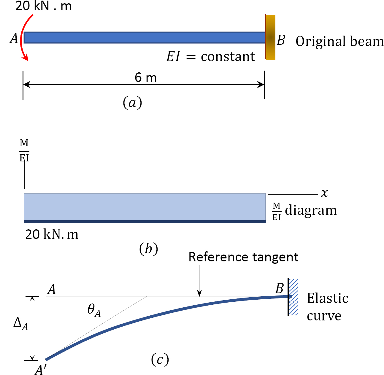
Example 7.7
A cantilever beam shown in Figure 7.10a is subjected to a concentrated moment at its free end. Using the moment-area method, determine the slope at the free end of the beam and the deflection at the free end of the beam. EI = constant.
Solution
(M/EI) diagram. First, draw the bending moment diagram for the beam and divide it by the flexural rigidity, EI, to obtain the  diagram shown in Figure 7.10b.
Slope at A. The slope at the free end is equal to the area of the diagram between A and B, according to the first moment-area theorem. Using this theorem and referring to the diagram suggests the following:


Example 7.8
A propped cantilever beam carries a uniformly distributed load of 4 kips/ft over its entire length, as shown in Figure 7.11a. Using the moment-area method, determine the slope at A and the deflection at A.

Solution
(M/EI) diagram. First, draw the bending moment diagram for the beam and divide it by the flexural rigidity, EI, to obtain the diagram shown in Figure 7.11b.
Slope at A. The slope at the free end is equal to the area of the diagram between A and B. The area between these two points is indicated as A1 and A2 in Figure 7.11b. Use Table 7.1 to find the computation of A2, whose arc is parabolic, and the location of its centroid. Noting from the table that 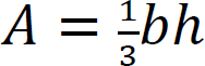 and applying the first moment-area theorem suggests the following:


Example 7.9
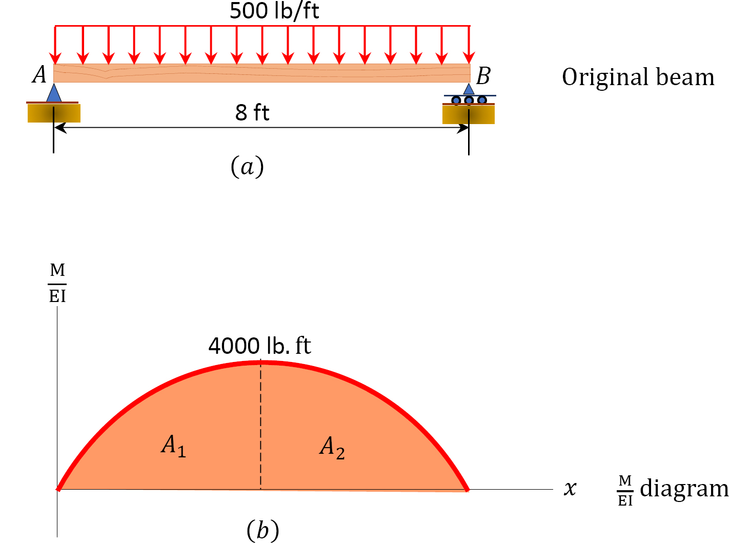
A simply supported timber beam with a length of 8 ft will carry a distributed floor load of 500 lb/ft over its entire length, as shown Figure 7.12a. Using the moment area theorem, determine the slope at end B and the maximum deflection.

Solution
(M/EI) diagram. First, draw the bending moment diagram for the beam, and divide it by the flexural rigidity, EI, to obtain the diagram shown in Figure 7.12b.
Slope at B. The slope at B is equal to the area of the diagram between B and C. The area between these two points is indicated as A2 in Figure 7.12b. Applying the first moment-area theorem suggests the following:

Maximum deflection. The maximum deflection occurs at the center of the beam (point C). It is equal to the moment of the area of the diagram between B and C about B. Thus,

Example 7.10
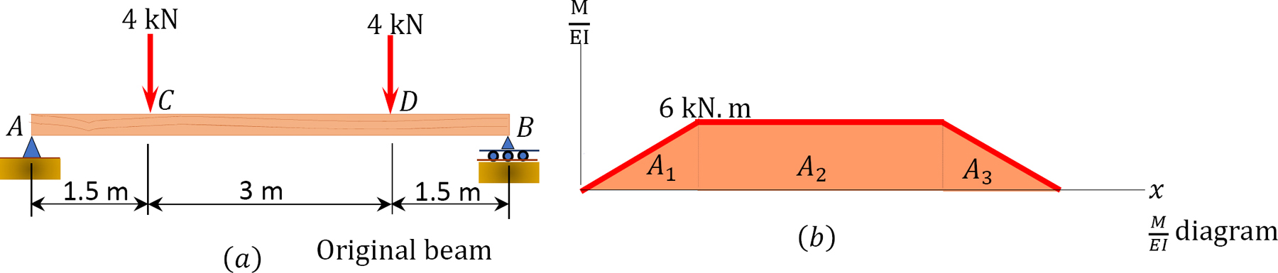
A prismatic timber beam is subjected to two concentrated loads of equal magnitude, as shown in Figure 7.13a. Using the moment-area method, determine the slope at A and the deflection at point C.

Solution
(M/EI) diagram. First, draw the bending moment diagram for the beam and divide it by the flexural rigidity, EI, to obtain the  diagram shown in Figure 7.13b.
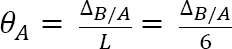
Slope at A. The deflection and the rotation of the beam are small since they occur within the elastic limit. Thus, the slope at support A can be computed using the small angle theorem, as follows:
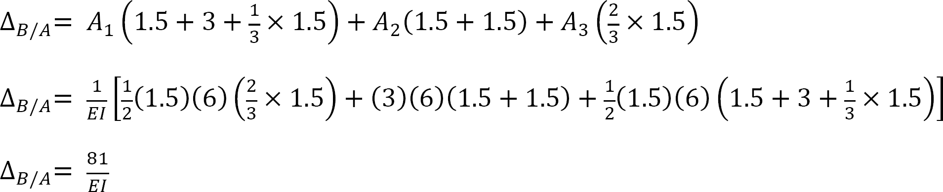
To determine the tangential deviation of B from A, apply the second moment-area theorem. According to the theorem, it is equal to the moment of the area of the diagram between A and B about B. Thus,
Thus, the slope at A is

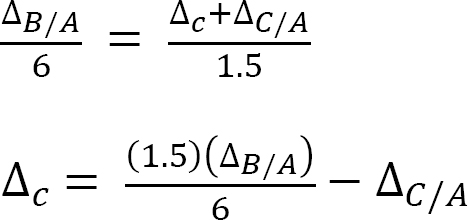
Deflection at C. The deflection at C can be obtained by proportion.
Similarly, the tangential deviation of C from A can be determined as the moment of the area of the  diagram between A and C about C.
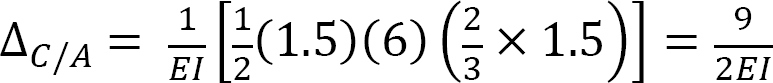
Therefore, the deflection at C is

7.6 Deflection by the Conjugate Beam Method
The conjugate beam method, developed by Heinrich Muller-Breslau in 1865, is one of the methods used to determine the slope and deflection of a beam. The method is based on the principle of statics.
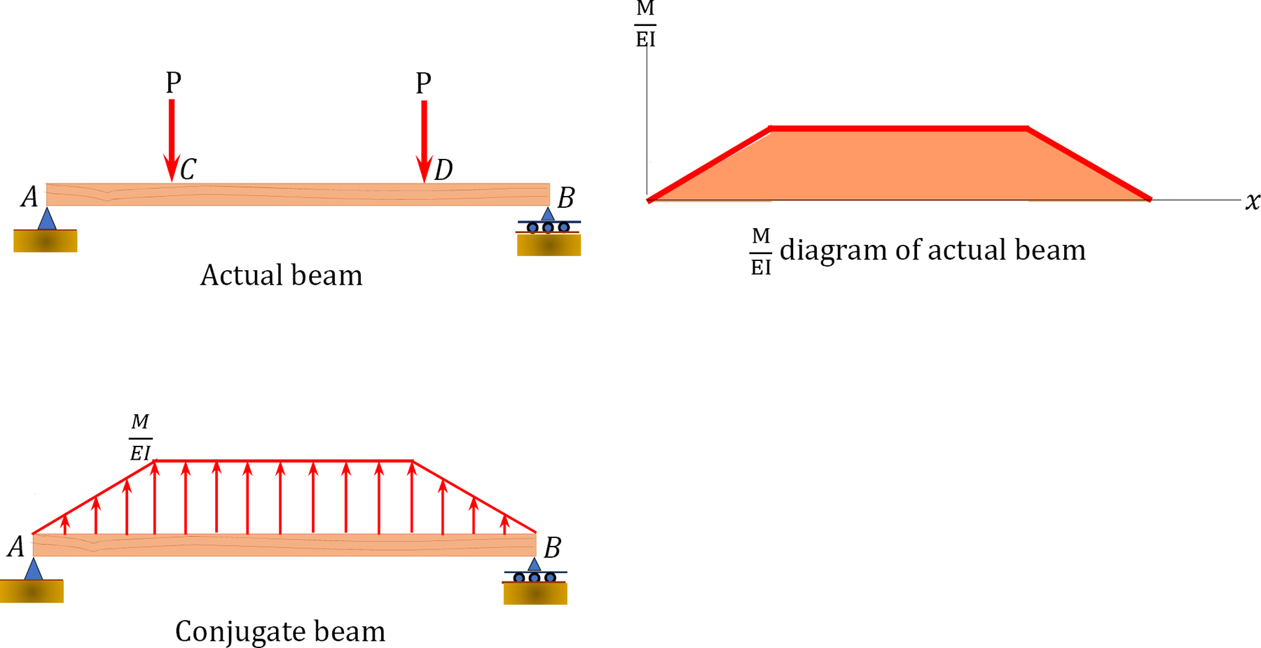
A conjugate beam is defined as a fictitious beam whose length is the same as that of the actual beam, but with a loading equal to the bending moment of the actual beam divided by its flexural rigidity, EI.
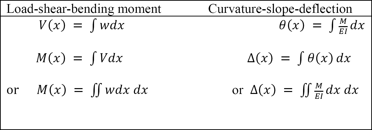
The conjugate beam method takes advantage of the similarity of the relationship among load, shear force, and bending moment, as well as among curvature, slope, and deflection derived in previous chapters and presented in Table 7.2.
Table 7.2. Relationship between load-shear-bending moment and curvature-slope-deflection.
7.6.1 Supports for Conjugate Beams
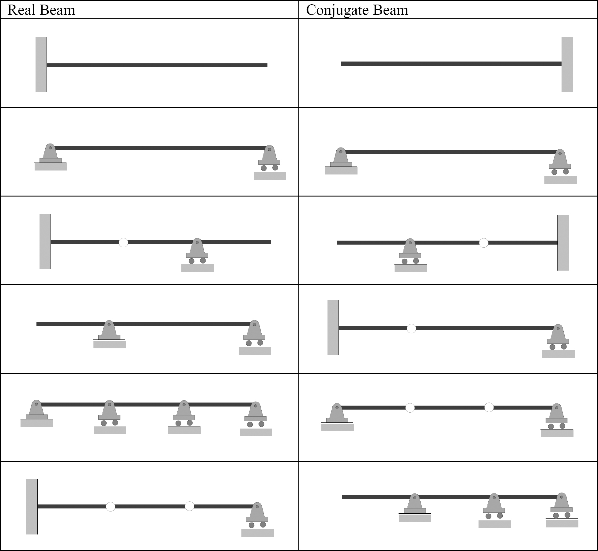
The supports for conjugate beams are shown in Table 7.3 and the examples of real and conjugate beams are shown in Figure 7.4.
Table 7.3. Supports for conjugate beams.
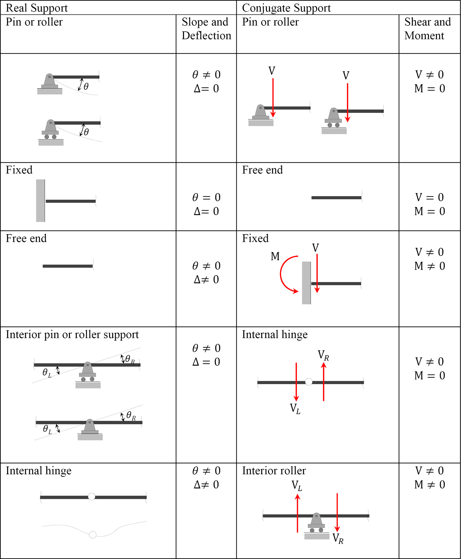
Table 7.4 Real beams and their conjugate.
7.6.2 Sign Convention
For a positive curvature diagram, where there is a positive ordinate of the  diagram, the load in the conjugate should point in the positive y direction (upward) and vice versa (see Figure 7.14).

If the convention stated for positive curvature diagrams is followed, then a positive shear force in the conjugate beam equals the positive slope in the real beam, and a positive moment in the conjugate beam equals a positive deflection (upward movement) of the real beam. This is shown in Figure 7.15.

Procedure for Analysis by Conjugate Beam Method
•Draw the curvature diagram for the real beam.
•Draw the conjugate beam for the real beam. The conjugate beam has the same length as the real beam. A rotation at any point in the real beam corresponds to a shear force at the same point in the conjugate beam, and a displacement at any point in the real beam corresponds to a moment in the conjugate beam.
•Apply the curvature diagram of the real beam as a distributed load on the conjugate beam.
•Using the equations of static equilibrium, determine the reactions at the supports of the conjugate beam.
•Determine the shear force and moment at the sections of interest in the conjugate beam. These shear forces and moments are equal to the slope and deflection, respectively, in the real beam. Positive shear in the conjugate beam implies a counterclockwise slope in the real beam, while a positive moment denotes an upward deflection in the real beam.
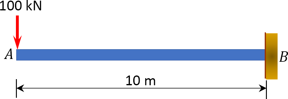
Example 7.11
Using the conjugate beam method, determine the slope and the deflection at point A of the cantilever beam shown in the Figure 7.16a. E = 29,000 ksi and I = 280 in.4

Solution
(M/EI) diagram. First, draw the bending moment diagram for the beam and divide it by the flexural rigidity, EI, to obtain the diagram shown in Figure 7.16b.
Conjugate beam. The conjugate beam loaded with the diagram is shown in Figure 7.16c. Notice that the free end in the real beam becomes fixed in the conjugate beam, while the fixed end in the real beam becomes free in the conjugate beam. The diagram is applied as a downward load in the conjugate beam because it is negative in Figure 7.16b.
Slope at A. The slope at A in the real beam is the shear at A in the conjugate beam. The shear at A in the conjugate is as follows:
The same sign convention for shear force used in Chapter 4 is used here.
Thus, the slope in the real beam at point A is as follows:

Deflection at A. The deflection at A in the real beam equals the moment at A of the conjugate beam. The moment at A of the conjugate beam is as follows:

The same sign convention for bending moment used in Chapter 4 is used here.
Thus, the deflection in the real beam at point A is as follows:

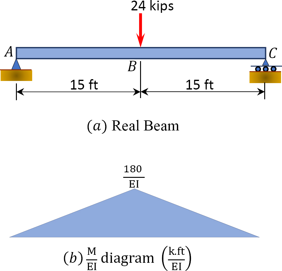
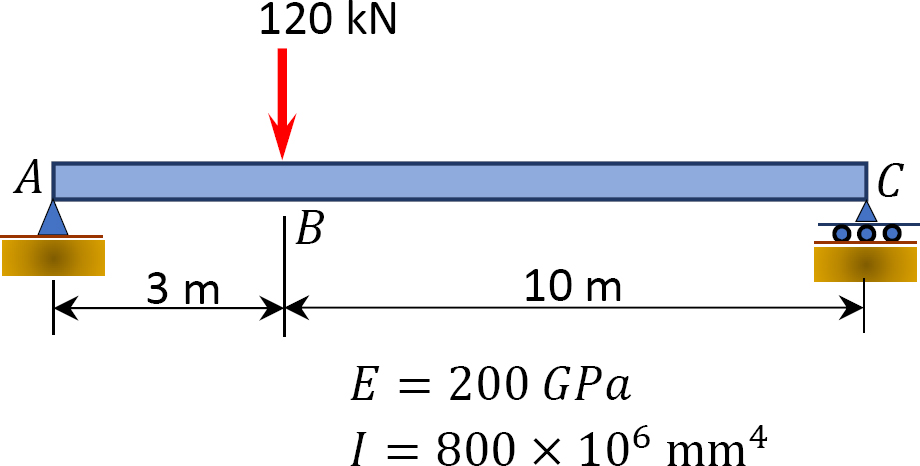
Example 7.12
Using the conjugate beam method, determine the slope at support A and the deflection under the concentrated load of the simply supported beam at B shown in Figure 7.17a.
E = 29,000 ksi and I = 800 in.4

Solution
(M/EI) diagram. First, draw the bending moment diagram for the beam and divide it by the flexural rigidity, EI, to obtain the moment curvature () diagram shown in Figure 7.17b.
Conjugate beam. The conjugate beam loaded with the diagram is shown in Figure 7.17c. Notice that A and C, which are simple supports in the real beam, remain the same in the conjugate beam. The diagram is applied as an upward load in the conjugate beam because it is positive in Figure 7.17b.
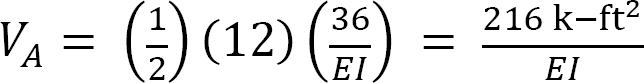
Reactions for conjugate beam. The reaction at supports of the conjugate beam can be determined as follows:

Slope at A. The slope at A in the real beam is the shear force at A in the conjugate beam. The shear at A in the conjugate beam is as follows:
Thus, the slope at support A of the real beam is as follows:

Deflection at B. The deflection at B in the real beam equals the moment at B of the conjugate beam. The moment at B of the conjugate beam is as follows:

The deflection at B of the real beam is as follows:

Chapter Summary
Deflection of beams through geometric methods: The geometric methods considered in this chapter includes the double integration method, singularity function method, moment-area method, and conjugate-beam method. Prior to discussion of these methods, the following equation of the elastic curve of a beam was derived:
Method of double integration: This method involves integrating the equation of elastic curve twice. The first integration yields the slope, and the second integration gives the deflection. The constants of integration are determined considering the boundary conditions.
Method of singularity function: This method involves using a singularity or half-range function to describe the equation of the elastic curve for the entire beam. A half-range function can be written in the general form as follows:
The method of singularity is best suited for beams with many discontinuities due to concentrated loads and moments. The method significantly reduces the number of constants of integration needed to be determined and, thus, makes computation easier when compared with the method of double integration.
Moment-area method: This method uses two theorems to determine the slope and deflection at specified points on the elastic curve of a beam. The two theorems are as follows:
First moment-area theorem: The change in slope between any two points on the elastic curve of a beam equals the area of the diagram between these two points.
Second moment-area theorem: The vertical deflection of point A from the tangent drawn to the elastic curve at point B equals the moment of the area under the diagram between these two points about point A.
Conjugate beam method: A conjugate beam has been defined as an imaginary beam with the same length as that of the actual beam but with a loading equal the diagram of the actual beam. The supports in the actual beams are replaced with fictitious supports with boundary conditions that will result in the bending moment and the shear force at a specific point in a conjugate beam equaling the deflection and slope, respectively, at the same points in the actual beam.
Practice Problems
7.1 Using the double integration method, determine the slopes and deflections at the free ends of the cantilever beams shown in Figure P7.1 through Figure P7.4. EI = constant.


7.2 Using the double integration method, determine the slopes at point A and the deflections at midpoint C of the beams shown in Figure P7.5 and Figure P7.6. EI = constant.


7.3 Using the conjugate beam method, determine the slope at point A and the deflection at point B of the beam shown in Figure P7.7 through Figure P7.10.


7.4 Using the moment-area method, determine the deflection at point A of the cantilever beam shown in Figure P7.11 through Figure P7.12.

7.5 Using the moment-area method, determine the slope at point A and the slope at the midpoint C of the beams shown in Figure P7.13 and Figure P7.14.


7.6 Using the method of singularity function, determine the slope and the deflection at point A of the cantilever beam shown in Figure P7.15.
7.7 Using the method of singularity function, determine the slope at point B and the slope at point C of the beam with the overhang shown in Figure P7.16. EI = constant. E = 200 GPa, I = 500 × 106 mm4.
7.8 Using the method of singularity function, determine the slope at point C and the deflection at point D of the beam with overhanging ends, as shown in Figure P7.17. EI = constant.

7.9 Using the method of singularity function, determine the slope at point A and the deflection at point B of the beam shown in Figure P7.18. EI = constant.
