2.4: Soil Mechanical Parameters

2.4.1. Grain Size Distribution/Particle Size Distribution

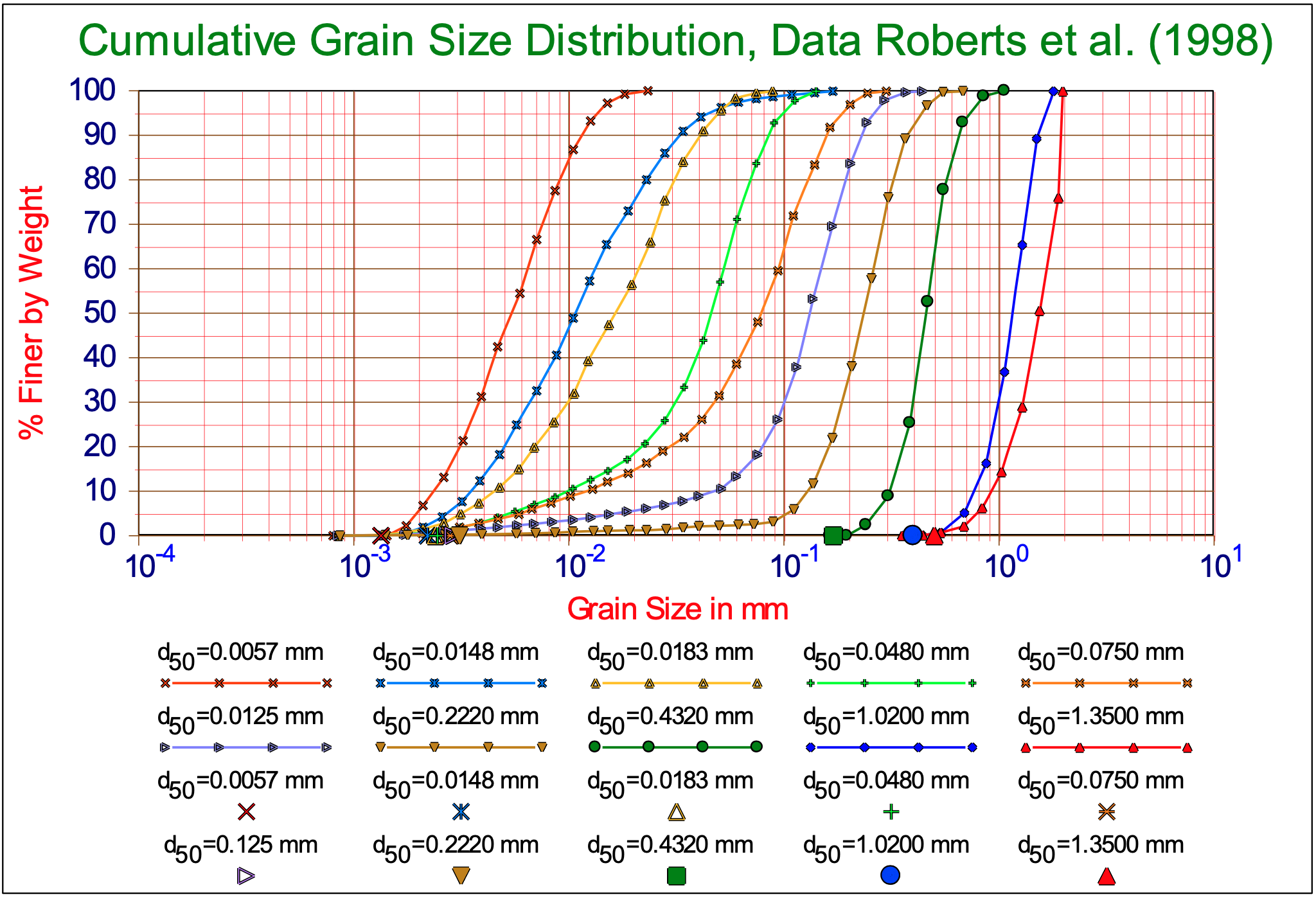
Soils consist of a mixture of particles of different size, shape and mineralogy. Because the size of the particles obviously has a significant effect on the soil behavior, the grain size and grain size distribution are used to classify soils. The grain size distribution describes the relative proportions of particles of various sizes. The grain size is often visualized in a cumulative distribution graph which, for example, plots the percentage of particles finer than a given size as a function of size. The median grain size, d50, is the size for which 50% of the particle mass consists of finer particles. Soil behavior, especially the hydraulic conductivity, tends to be dominated by the smaller particles; hence, the term "effective size", denoted by d10, is defined as the size for which 10% of the particle mass consists of finer particles.

Sands and gravels that possess a wide range of particle sizes with a smooth distribution of particle sizes are called well graded soils. If the soil particles in a sample are predominantly in a relatively narrow range of sizes, the soil is called uniformly graded soils. If there are distinct gaps in the gradation curve, e.g., a mixture of gravel and fine sand, with no coarse sand, the soils may be called gap graded. Uniformly graded and gap graded soils are both considered to be poorly graded. There are many methods for measuring particle size distribution. The two traditional methods used in geotechnical engineering are sieve analysis and hydrometer analysis.

Figure 2-18: The particle size distributions of the sands used by Roberts et al. (1998).

2.4.2. Atterberg Limits

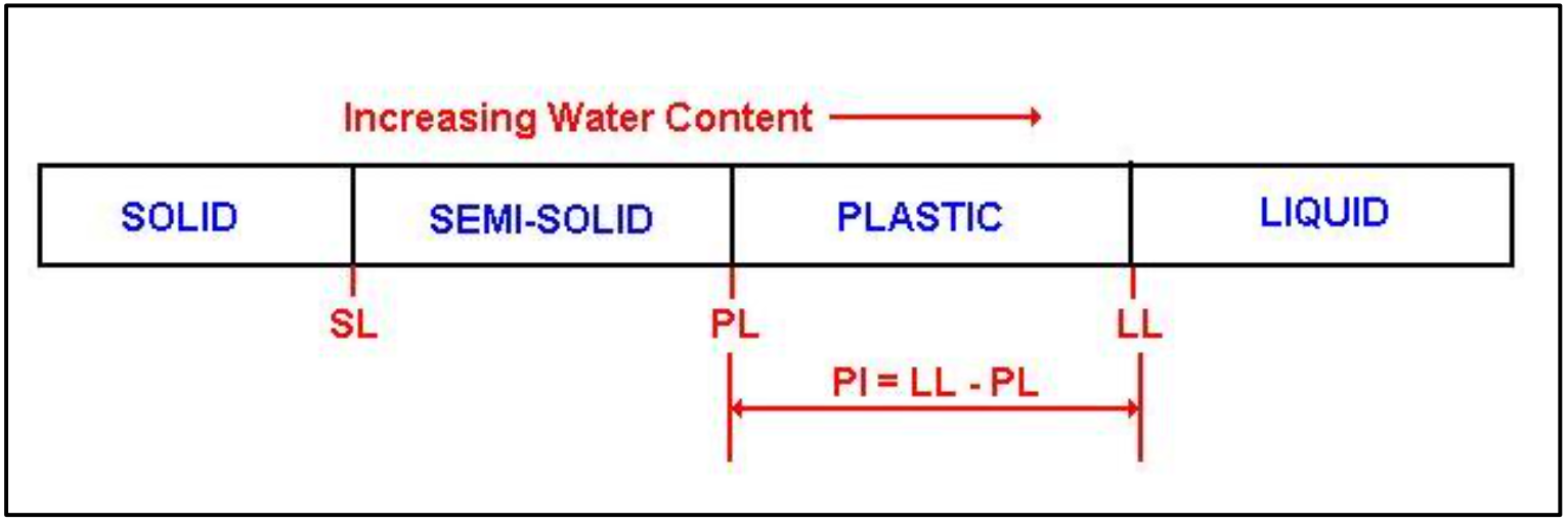
The Atterberg limits are a basic measure of the nature of a fine-grained soil. Depending on the water content of the soil, it may appear in four states: solid, semi-solid, plastic and liquid. In each state the consistency and behavior of a soil is different and thus so are its engineering properties. Thus, the boundary between each state can be defined based on a change in the soil's behavior. The Atterberg limits can be used to distinguish between silt and clay, and it can distinguish between different types of silts and clays. These limits were created by Albert Atterberg, a Swedish chemist. They were later refined by Arthur Casagrande. These distinctions in soil are used in picking the soils to build structures on top of. These tests are mainly used on clayey or silty soils since these are the soils that expand and shrink due to moisture content. Clays and silts react with the water and thus change sizes and have varying shear strengths. Thus these tests are used widely in the preliminary stages of building any structure to insure that the soil will have the correct amount of shear strength and not too much change in volume as it expands and shrinks with different moisture contents.

Figure 2-19: Liquid limit device.

Figure 2-20: Liquid limit device.

2.4.2.1. Shrinkage Limit

The shrinkage limit (SL) is the water content where further loss of moisture will not result in any more volume reduction. The test to determine the shrinkage limit is ASTM International D4943. The shrinkage limit is much less commonly used than the liquid and plastic limits.

2.4.2.2. Plastic Limit

The plastic limit (PL) is the water content where soil transitions between brittle and plastic behavior. A thread of soil is at its plastic limit when it begins to crumble when rolled to a diameter of 3 mm. To improve test result consistency, a 3 mm diameter rod is often used to gauge the thickness of the thread when conducting the test. The Plastic Limit test is defined by ASTM standard test method D 4318.

2.4.2.3. Liquid Limit

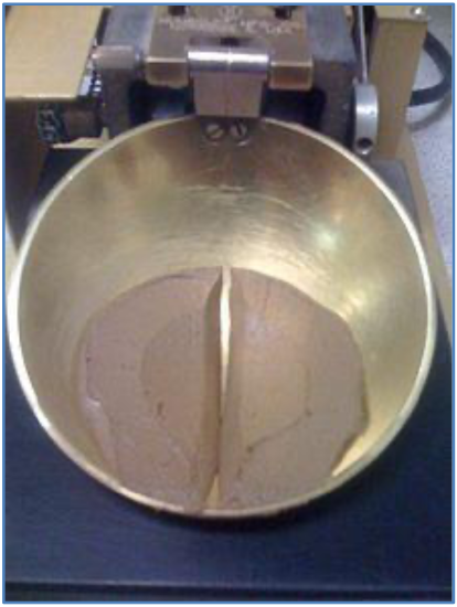
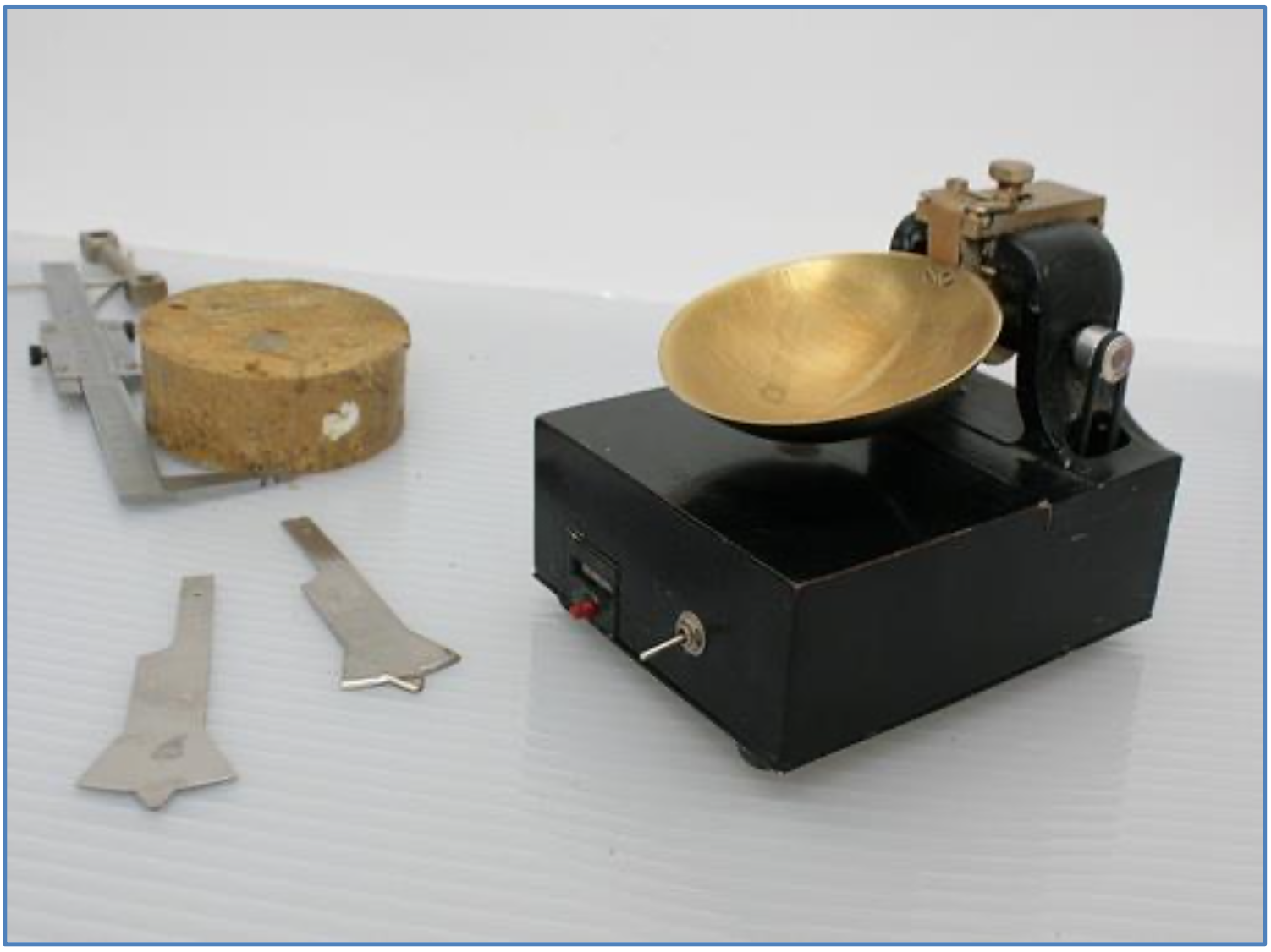
The liquid limit (LL) is the water content at which a soil changes from plastic to liquid behavior. The original liquid limit test of Atterberg's involved mixing a pat of clay in a round-bottomed porcelain bowl of 10-12cm diameter. A groove was cut through the pat of clay with a spatula, and the bowl was then struck many times against the palm of one hand. Casagrande subsequently standardized the apparatus and the procedures to make the measurement more repeatable. Soil is placed into the metal cup portion of the device and a groove is made down its center with a standardized tool of 13.5 millimeters (0.53 in) width. The cup is repeatedly dropped 10mm onto a hard rubber base during which the groove closes up gradually as a result of the impact. The number of blows for the groove to close is recorded. The moisture content at which it takes 25 drops of the cup to cause the groove to close over a distance of 13.5 millimeters (0.53 in) is defined as the liquid limit. The test is normally run at several moisture contents, and the moisture content which requires 25 blows to close the groove is interpolated from the test results. The Liquid Limit test is defined by ASTM standard test method D 4318. The test method also allows running the test at one moisture content where 20 to 30 blows are required to close the groove; then a correction factor is applied to obtain the liquid limit from the moisture content.

The following is when you should record the N in number of blows needed to close this 1/2-inch gap: The materials needed to do a Liquid limit test are as follows

• Casagrande cup ( liquid limit device)

• Grooving tool

• Soil pat before test

• Soil pat after test

Another method for measuring the liquid limit is the fall cone test. It is based on the measurement of penetration into the soil of a standardized cone of specific mass. Despite the universal prevalence of the Casagrande method, the fall cone test is often considered to be a more consistent alternative because it minimizes the possibility of human variations when carrying out the test.

2.4.2.4. Importance of Liquid Limit Test

The importance of the liquid limit test is to classify soils. Different soils have varying liquid limits. Also to find the plasticity index of a soil you need to know the liquid limit and the plastic limit.

2.4.2.5. Derived Limits

The values of these limits are used in a number of ways. There is also a close relationship between the limits and properties of a soil such as compressibility, permeability, and strength. This is thought to be very useful because as limit determination is relatively simple, it is more difficult to determine these other properties. Thus the Atterberg limits are not only used to identify the soil's classification, but it allows for the use of empirical correlations for some other engineering properties.

2.4.2.6. Plasticity Index

The plasticity index (PI) is a measure of the plasticity of a soil. The plasticity index is the size of the range of water contents where the soil exhibits plastic properties. The PI is the difference between the liquid limit and the plastic limit (PI = LL-PL). Soils with a high PI tend to be clay, those with a lower PI tend to be silt, and those with a PI of 0 (non-plastic) tend to have little or no silt or clay.

PI and their meanings

• 0 – Non-plastic

• (1-5)- Slightly Plastic

• (5-10) - Low plasticity

• (10-20)- Medium plasticity

• (20-40)- High plasticity

• >40 Very high plasticity

2.4.2.7. Liquidity Index

The liquidity index (LI) is used for scaling the natural water content of a soil sample to the limits. It can be calculated as a ratio of difference between natural water content, plastic limit, and plasticity index: LI=(W-PL)/(LL-PL) where W is the natural water content.

2.4.2.8. Activity

The activity (A) of a soil is the PI divided by the percent of clay-sized particles (less than 2 μm) present. Different types of clays have different specific surface areas which controls how much wetting is required to move a soil from one phase to another such as across the liquid limit or the plastic limit. From the activity one can predict the dominant clay type present in a soil sample. High activity signifies large volume change when wetted and large shrinkage when dried. Soils with high activity are very reactive chemically. Normally the activity of clay is between 0.75 and 1.25, and in this range clay is called normal. It is assumed that the plasticity index is approximately equal to the clay fraction (A = 1). When A is less than 0.75, it is considered inactive. When it is greater than 1.25, it is considered active.

Figure 2-21: The relation between SL, PL, LL and PI.

2.4.3. Mass Volume Relations

There are a variety of parameters used to describe the relative proportions of air (gas), water (liquid) and solids in a soil. This section defines these parameters and some of their interrelationships. The basic notation is as follows:

V_g, V_l, and V_s represent the volumes of gas, liquid and solids in a soil mixture;

W_g, W_l, and W_s represent the weights of gas, liquid and solids in a soil mixture;

M_g, M_l, and M_s represent the masses of gas, liquid and solids in a soil mixture;

ρ_g, ρ_l, and ρ_s represent the densities of the constituents (gas, liquid and solids) in a soil mixture;

Note that the weights, W, can be obtained by multiplying the mass, M, by the acceleration due to gravity, g; e.g., W_s = M_s·g

2.4.3.1. Specific Gravity

Specific Gravity is the ratio of the density of one material compared to the density of pure water (ρ_l = 1000 kg/m³).

\[\ \mathrm{G}_{\mathrm{s}}=\frac{\rho_{\mathrm{s}}}{\rho_{\mathrm{l}}}\tag{2-1}\]

2.4.3.2. Density

The terms density and unit weight are used interchangeably in soil mechanics. Though not critical, it is important that we know it. Density, Bulk Density, or Wet Density, ρ_t, are different names for the density of the mixture, i.e., the total mass of air, water, solids divided by the total volume of air, water and solids (the mass of air is assumed to be zero for practical purposes. To find the formula for density, divide the mass of the soil by the volume of the soil, the basic formula for density is:

\[\ \mathrm{ \rho_{t}=\frac{M_{t}}{V_{t}}=\frac{M_{s}+M_{l}+M_{g}}{V_{s}+V_{l}+V_{g}}}\tag{2-2}\]

Unit weight of a soil mass is the ratio of the total weight of soil to the total volume of soil. Unit Weight, \(\ \gamma_t\), is usually determined in the laboratory by measuring the weight and volume of a relatively undisturbed soil sample obtained from a brass ring. Measuring unit weight of soil in the field may consist of a sand cone test, rubber balloon or nuclear densitometer, the basic formula for unit weight is:

\[\ \gamma_{\mathrm{t}}=\frac{\mathrm{M}_{\mathrm{t}} \cdot \mathrm{g}}{\mathrm{V}_{\mathrm{t}}}\tag{2-3}\]

Dry Density, ρ_d, is the mass of solids divided by the total volume of air, water and solids:

\[\ \rho_{\mathrm{d}}=\frac{\mathrm{M}_{\mathrm{s}}}{\mathrm{V}_{\mathrm{t}}}=\frac{\mathrm{M}_{\mathrm{s}}}{\mathrm{V}_{\mathrm{s}}+\mathrm{V}_{\mathrm{l}}+\mathrm{V}_{\mathrm{g}}}\tag{2-4}\]

Submerged Density, ρ_st, defined as the density of the mixture minus the density of water is useful if the soil is submerged under water:

\[\ \rho_{\mathrm{sd}}=\rho_{\mathrm{t}}-\rho_{\mathrm{l}}\tag{2-5}\]

Table 2-2: Empirical values for ρ_t, of granular soils based on the standard penetration number, (from Bowels, Foundation Analysis).

SPT Penetration, N-Value (blows/ foot)	ρt (kg/m^3)
0-4	1120 - 1520
4 - 10	1520 - 1800
10 - 30	1800 - 2080
30 - 50	2080 - 2240
>50	2240 - 2400

Table 2-3: Empirical values for ρ_s, of cohesive soils based on the standard penetration number, (From Bowels, Foundation Analysis).

SPT Penetration, N-Value (blows/ foot)	ρs, sat (kg/m^3)
0 - 4	1600 - 1840
4 - 8	1840 - 2000
8 - 32	2000 - 2240

Table 2-4: Typical Soil Characteristics (From Lindeburg, Civil Engineering Reference Manual for the PE Exam, 8^th edition).

Soil Type	ρs (kg/m^3)	ρs, sat (kg/m^3)
Sand, loose and uniform	1440	1888
Sand, dense and uniform	1744	2080
Sand, loose and well graded	1584	1984
Sand, dense and well graded	1856	2160
Glacial clay, soft	1216	1760
Glacial clay, stiff	1696	2000

Table 2-5: Typical Values of Soil Index Properties (From NAVFAC 7.01).

Soil Type	ρs (kg/m^3)
Sand; clean, uniform, fine or medium	1344 - 2176
Silt; uniform, inorganic	1296 - 2176
Silty Sand	1408 - 2272
Sand; Well-graded	1376 - 2368
Silty Sand and Gravel	1440 - 2480
Sandy or Silty Clay	1600 - 2352
Silty Clay with Gravel; uniform	1840 - 2416
Well-graded Gravel, Sand, Silt and Clay	2000 - 2496
Clay	1504 - 2128
Colloidal Clay	1136 - 2048
Organic Silt	1392 - 2096
Organic Clay	1296 - 2000

2.4.3.3. Relative Density.

Relative density is an index that quantifies the state of compactness between the loosest and densest possible state of coarse-grained soils. The relative density is written in the following formulas:

\[\ \mathrm{D}_{\mathrm{r}}=\frac{\mathrm{e}_{\mathrm{m a x}}-\mathrm{e}}{\mathrm{e}_{\mathrm{m a x}}-\mathrm{e}_{\mathrm{m i n}}}=\frac{\mathrm{n}_{\mathrm{m a x}}-\mathrm{n}}{\mathrm{n}_{\mathrm{m a x}}-\mathrm{n}_{\mathrm{m i n}}}\tag{2-6}\]

Table 2-6: Designation of Granular Soil Based on Relative Density.

Dr (%)	Description
0 - 20	Very loose
20 - 40	Loose
40 - 70	Medium dense
70 - 85	Dense
85 - 100	Very dense

Figure 2-22: SPT values versus relative density (Miedema (1995).

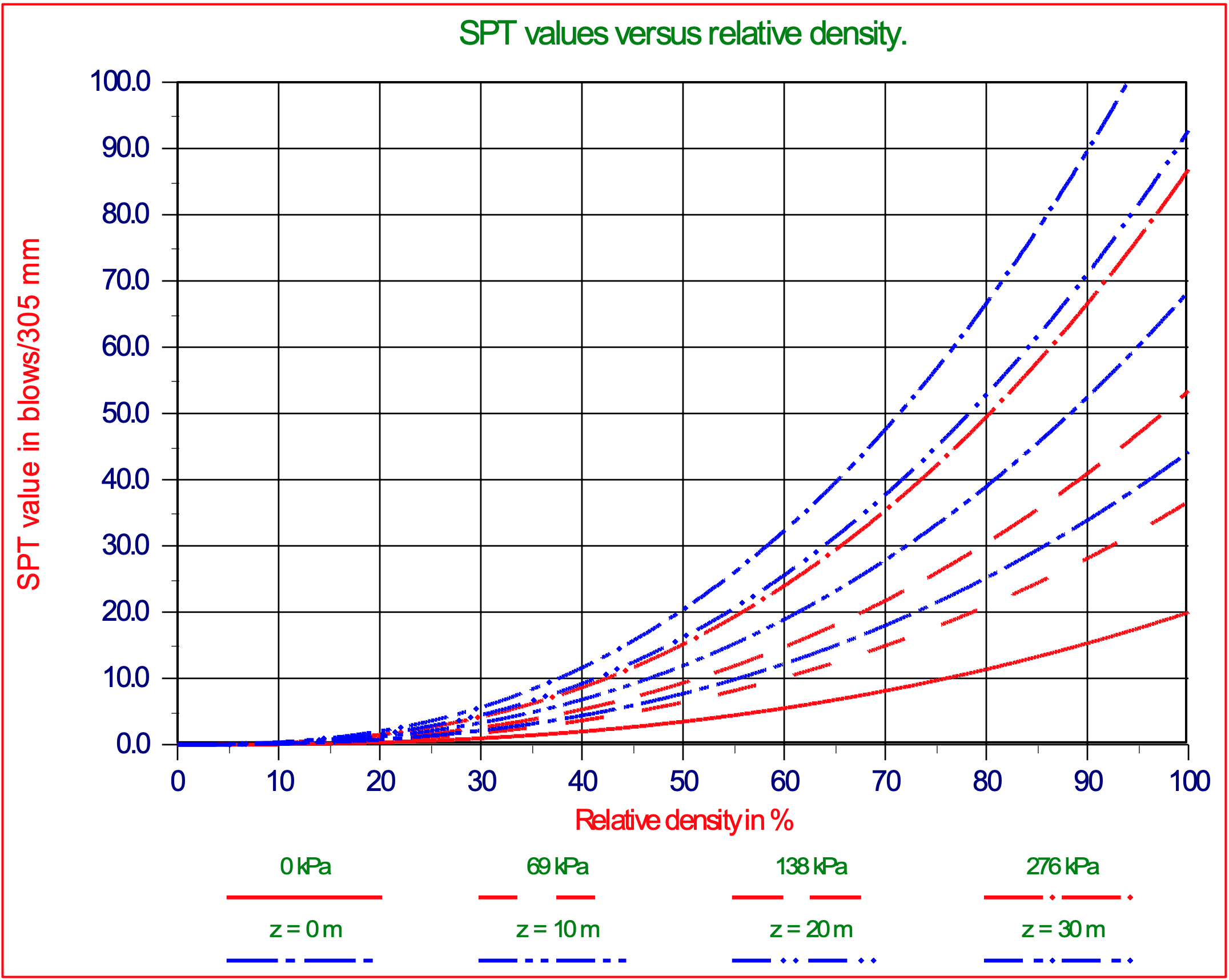
Lambe & Whitman (1979), page 78 (Figure 2-22) give the relation between the SPT value, the relative density and the hydrostatic pressure in two graphs. With some curve-fitting these graphs can be summarized with the following equation (Miedema (1995)):

\[\ \operatorname{SPT}=(1.82+0.221 \cdot(z+10)) \cdot 10^{-4} \cdot \mathrm{RD}^{2.52}\tag{2-7}\]

2.4.3.4. Porosity

Porosity is the ratio of the volume of openings (voids) to the total volume of material. Porosity represents the storage capacity of the geologic material. The primary porosity of a sediment or rock consists of the spaces between the grains that make up that material. The more tightly packed the grains are, the lower the porosity. Using a box of marbles as an example, the internal dimensions of the box would represent the volume of the sample. The space surrounding each of the spherical marbles represents the void space. The porosity of the box of marbles would be determined by dividing the total void space by the total volume of the sample and expressed as a percentage.

The primary porosity of unconsolidated sediments is determined by the shape of the grains and the range of grain sizes present. In poorly sorted sediments, those with a larger range of grain sizes, the finer grains tend to fill the spaces between the larger grains, resulting in lower porosity. Primary porosity can range from less than one percent in crystalline rocks like granite to over 55% in some soils. The porosity of some rock is increased through fractures or solution of the material itself. This is known as secondary porosity.

\[\ \mathrm{n}=\frac{\mathrm{V}_{\mathrm{v}}}{\mathrm{V}_{\mathrm{t}}}=\frac{\mathrm{V}_{\mathrm{v}}}{\mathrm{V}_{\mathrm{s}}+\mathrm{V}_{\mathrm{v}}}=\frac{\mathrm{e}}{1+\mathrm{e}}\tag{2-8}\]

2.4.3.5. Void ratio

The ratio of the volume of void space to the volume of solid substance in any material consisting of void space and solid material, such as a soil sample, a sediment, or a powder.

\[\ \mathrm{e}=\frac{\mathrm{V}_{\mathrm{v}}}{\mathrm{V}_{\mathrm{s}}}=\frac{\mathrm{V}_{\mathrm{v}}}{\mathrm{V}_{\mathrm{t}}-\mathrm{V}_{\mathrm{v}}}=\frac{\mathrm{n}}{1-\mathrm{n}}\tag{2-9}\]

The relations between void ratio e and porosity n are:

\[\ \mathrm{e}=\frac{\mathrm{n}}{1-\mathrm{n}} \quad\text{ and }\quad \mathrm{n}=\frac{\mathrm{e}}{1+\mathrm{e}}\tag{2-10}\]

2.4.3.6. Dilatation

Dilation (or dilatation) refers to an enlargement or expansion in bulk or extent, the opposite of contraction. It derives from the Latin dilatare, "to spread wide". It is the increase in volume of a granular substance when its shape is changed, because of greater distance between its component particles. Suppose we have a volume V before the enlargement and a volume V+dV after the enlargement. Before the enlargement we name the porosity n_i (i from initial) and after the enlargement n_cv (the constant volume situation after large deformations). For the volume before the deformation we can write:

\[\ \mathrm{V}=\left(1-\mathrm{n}_{\mathrm{i}}\right) \cdot \mathrm{V}+\mathrm{n}_{\mathrm{i}} \cdot \mathrm{V}\tag{2-11}\]

The first term on the right hand side is the sand volume, the second term the pore volume. After the enlargement we get:

\[\ \mathrm{V}+\mathrm{d V}=\left(\mathrm{1 - n}_{\mathrm{c v}}\right) \cdot(\mathrm{V}+\mathrm{d} \mathrm{V})+\mathrm{n}_{\mathrm{c v}} \cdot(\mathrm{V}+\mathrm{d} \mathrm{V})\tag{2-12}\]

Again the first term on the right hand side is the sand volume. Since the sand volume did not change during the enlargement (we assume the quarts grains are incompressible), the volume of sand in both equations should be the same, thus:

\[\ \mathrm{\left(1-n_{i}\right) \cdot V=\left(1-n_{c v}\right) \cdot(V+d V)}\tag{2-13}\]

From this we can deduce that the dilatation ε is:

\[\ \varepsilon=\frac{\mathrm{d} \mathrm{V}}{\mathrm{V}}=\frac{\mathrm{n}_{\mathrm{c} \mathrm{v}}-\mathrm{n}_{\mathrm{i}}}{\mathrm{1}-\mathrm{n}_{\mathrm{c} \mathrm{v}}}=\frac{\mathrm{d n}}{\mathrm{1}-\mathrm{n}_{\mathrm{c} \mathrm{v}}}\tag{2-14}\]

2.4.4. Permeability

Permeability is a measure of the ease with which fluids will flow though a porous rock, sediment, or soil. Just as with porosity, the packing, shape, and sorting of granular materials control their permeability. Although a rock may be highly porous, if the voids are not interconnected, then fluids within the closed, isolated pores cannot move. The degree to which pores within the material are interconnected is known as effective porosity. Rocks such as pumice and shale can have high porosity, yet can be nearly impermeable due to the poorly interconnected voids. In contrast, well-sorted sandstone closely replicates the example of a box of marbles cited above. The rounded sand grains provide ample, unrestricted void spaces that are free from smaller grains and are very well linked. Consequently, sandstones of this type have both high porosity and high permeability.

The range of values for permeability in geologic materials is extremely large. The most conductive materials have permeability values that are millions of times greater than the least permeable. Permeability is often directional in nature. The characteristics of the interstices of certain materials may cause the permeability to be significantly greater in one direction. Secondary porosity features, like fractures, frequently have significant impact on the permeability of the material. In addition to the characteristics of the host material, the viscosity and pressure of the fluid also affect the rate at which the fluid will flow.

Hydraulic conductivity or permeability k can be estimated by particle size analysis of the sediment of interest, using empirical equations relating either k to some size property of the sediment. Vukovic and Soro (1992) summarized several empirical methods from former studies and presented a general formula:

\[\ \mathrm{k}=\mathrm{C} \cdot \frac{\mathrm{g}}{v_{\mathrm{l}}} \cdot \mathrm{f}(\mathrm{n}) \cdot \mathrm{d}_{\mathrm{e}}^{\mathrm{2}}\tag{2-15}\]

The kinematic viscosity v_l is related to dynamic viscosity μ_l and the fluid (water) density ρ_l as follows:

\[\ v_{\mathrm{l}}=\frac{\mu_{\mathrm{l}}}{\rho_{\mathrm{l}}}\tag{2-16}\]

The values of C, f(n) and d_e are dependent on the different methods used in the grain-size analysis. According to Vukovic and Soro (1992), porosity n may be derived from the empirical relationship with the coefficient of grain uniformity U as follows:

\[\ \mathrm{n}=\mathrm{0 .2 5 5} \cdot\left(\mathrm{1}+\mathrm{0 .8 3}^{\mathrm{U}}\right)\tag{2-17}\]

Where U is the coefficient of grain uniformity and is given by:

\[\ \mathrm{U}=\left(\frac{\mathrm{d}_{\mathrm{60}}}{\mathrm{d}_{\mathrm{10}}}\right)\tag{2-18}\]

Here, d₆₀ and d₁₀ in the formula represent the grain diameter in (mm) for which, 60% and 10% of the sample respectively, are finer than. Former studies have presented the following formulae which take the general form presented in equation (2-15) above but with varying C, f(n) and d_e values and their domains of applicability.

Hazen’s formula (1982) was originally developed for determination of hydraulic conductivity of uniformly graded sand but is also useful for fine sand to gravel range, provided the sediment has a uniformity coefficient less than 5 and effective grain size between 0.1 and 3mm.

\[\ \mathrm{k}=\mathrm{6} \cdot \mathrm{1 0}^{-4} \cdot \frac{\mathrm{g}}{v_{\mathrm{l}}} \cdot(1+\mathrm{1 0} \cdot(\mathrm{n}-\mathrm{0} . \mathrm{2 6})) \cdot \mathrm{d}_{10}^{2}\tag{2-19}\]

The Kozeny-Carman equation is one of the most widely accepted and used derivations of permeability as a function of the characteristics of the soil medium. The Kozeny-Carman equation (or Carman-Kozeny equation) is a relation used in the field of fluid dynamics to calculate the pressure drop of a fluid flowing through a packed bed of solids. It is named after Josef Kozeny and Philip C. Carman. This equation was originally proposed by Kozeny (1927) and was then modified by Carman (1937) and (1956) to become the Kozeny-Carman equation. It is not appropriate for either soil with effective size above 3 mm or for clayey soils. The equation is only valid for laminar flow. The equation is given as:

\[\ \begin{array}{left}\mathrm{k}=\mathrm{d}_{\mathrm{e}}^{2} \cdot \frac{\gamma_{\mathrm{l}}}{\mu_{\mathrm{l}}} \cdot \frac{\mathrm{e}^{\mathrm{3}}}{\mathrm{1}+\mathrm{e}} \cdot \mathrm{C} \quad\text{ or }\quad \mathrm{k}=\mathrm{8.3} \cdot \mathrm{10}^{-\mathrm{3}} \cdot \frac{\mathrm{g}}{v_{\mathrm{l}}} \cdot \frac{\mathrm{n}^{\mathrm{3}}}{(\mathrm{1}-\mathrm{n})^{2}} \cdot \mathrm{d}_{10}^{2}\\
\text{With: }\quad v_{\mathrm{l}}=\frac{\mu_{\mathrm{l}}}{\rho_{\mathrm{l}}}\quad\text{ and }\quad\gamma_{\mathrm{l}}=\rho_{\mathrm{l}} \cdot \mathrm{g}\end{array}\tag{2-20}\]

This equation holds for flow through packed beds with particle Reynolds numbers up to approximately 1.0, after which point frequent shifting of flow channels in the bed causes considerable kinetic energy losses. This equation can be expressed as "flow is proportional to the pressure drop and inversely proportional to the fluid viscosity", which is known as Darcy's law.

The Breyer method does not consider porosity and therefore, porosity function takes on value 1. Breyer formula is often considered most useful for materials with heterogeneous distributions and poorly sorted grains with uniformity coefficient between 1 and 20, and effective grain size between 0.06mm and 0.6mm.

\[\ \mathrm{k}=\mathrm{6} \cdot \mathrm{1 0}^{-4} \cdot \frac{\mathrm{g}}{v_{\mathrm{l}}} \cdot \log \left(\frac{\mathrm{5 0 0}}{\mathrm{U}}\right) \cdot \mathrm{d}_{10}^{2}\tag{2-21}\]

The Slitcher formula is most applicable for grain-sizes between 0.01 mm and 5 mm.

\[\ \mathrm{k}=\mathrm{1} \cdot \mathrm{1 0}^{-\mathrm{2}} \cdot \frac{\mathrm{g}}{v_{\mathrm{l}}} \cdot \mathrm{n}^{\mathrm{3.287}} \cdot \mathrm{d}_{\mathrm{1 0}}^{\mathrm{2}}\tag{2-22}\]

The Terzaghi (1964) formula is most applicable for coarse sand. The Terzaghi equation:

\[\ \mathrm{k}=\mathrm{C}_{\mathrm{t}} \cdot \frac{\mathrm{g}}{v_{\mathrm{l}}} \cdot\left(\frac{\mathrm{n}-\mathrm{0 .1 3}}{\sqrt[3]{\mathrm{1 - n}}}\right)^{2} \cdot \mathrm{d}_{\mathrm{1 0}}^{\mathrm{2}}\tag{2-23}\]

Where the C_t = sorting coefficient and 6.1 x 10^-3 < C_t < 10.7 x 10^-3. 

2.4.5. The Angle of Internal Friction

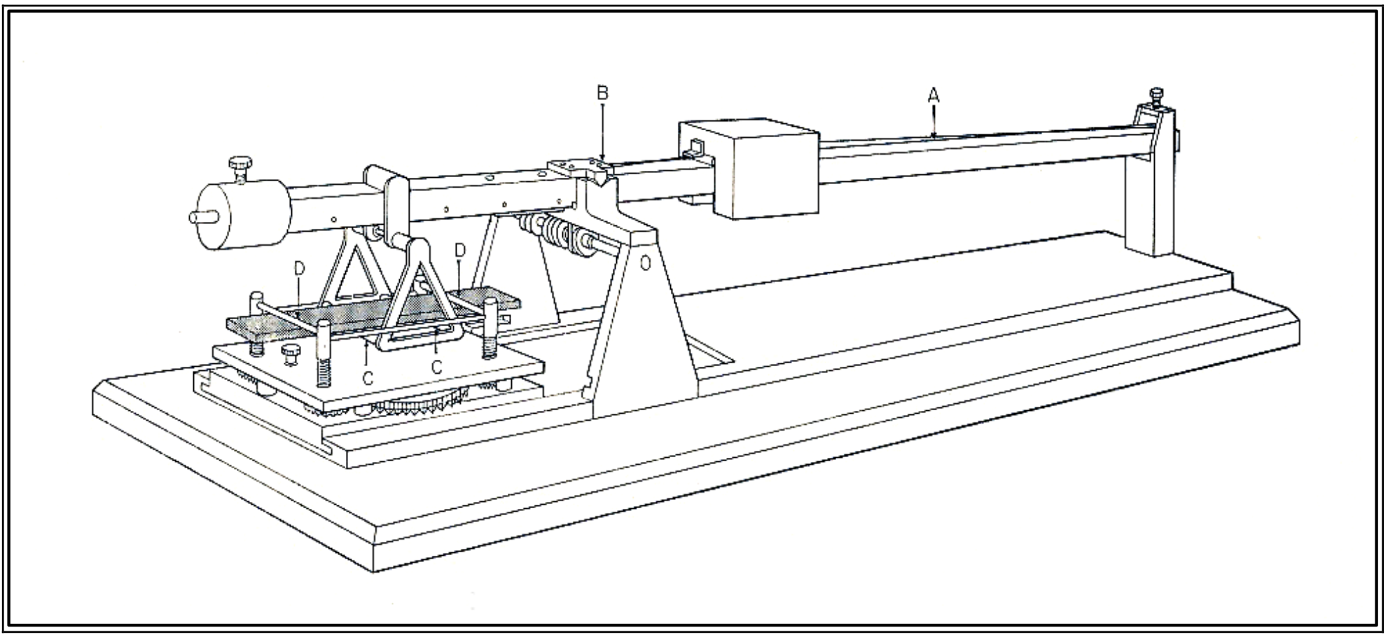
Angle of internal friction for a given soil is the angle on the graph (Mohr's Circle) of the shear stress and normal effective stresses at which shear failure occurs. Angle of Internal Friction, φ, can be determined in the laboratory by the Direct Shear Test or the Triaxial Stress Test. Typical relationships for estimating the angle of internal friction, φ, are as follows:

Table 2-7: Empirical values for φ, of granular soils based on the standard penetration number, (From Bowels, Foundation Analysis).

SPT Penetration, N-Value (blows/ foot)	φ (degrees)
0	25-30
4	27-32
10	30-35
30	35-40
50	38-43

Table 2-8: Relationship between φ, and standard penetration number for sands, (From Peck 1974, Foundation Engineering Handbook).

SPT Penetration, N-Value (blows/ foot)	Density of Sand	φ (degrees)
<4	Very loose	<29
4 - 10	Loose	29 - 30
10 - 30	Medium	30 - 36
30 - 50	Dense	36 - 41
>50	Very dense	>41

Table 2-9: Relationship between φ, and standard penetration number for sands, (From Meyerhof 1956, Foundation Engineering Handbook).

SPT Penetration, N-Value (blows/ foot)	Density of Sand	φ (degrees)
<4	Very loose	<30
4 - 10	Loose	30 - 35
10 - 30	Medium	35 - 40
30 - 50	Dense	40 - 45
>50	Very dense	>45

Lambe & Whitman (1979), page 148 (Figure 2-23) give the relation between the SPT value and the angle of internal friction, also in a graph. This graph is valid up to 12 m in dry soil. With respect to the internal friction, the relation given in the graph has an accuracy of 3 degrees. A load of 12 m dry soil with a density of 1.67 ton/m3 equals a hydrostatic pressure of 20 m.w.c. An absolute hydrostatic pressure of 20 m.w.c. equals 10 m of water depth if cavitation is considered. Measured SPT values at any depth will have to be reduced to the value that would occur at 10 m water depth. This can be accomplished with the following equation:

\[\ \operatorname{SPT}_{10}=\frac{1}{(0.646+0.0354 \cdot \mathrm{z})} \cdot \mathrm{SPT}_{\mathrm{z}}\tag{2-24}\]

Figure 2-23: Friction angle versus SPT value (Miedema (1995).

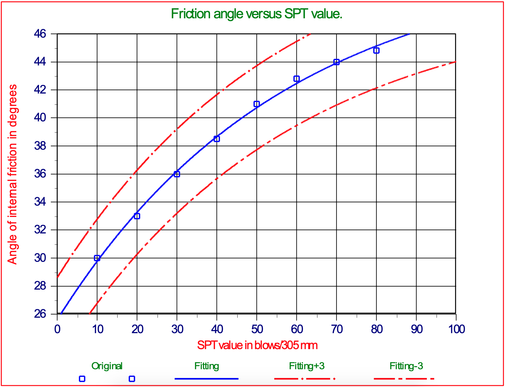
With the aim of curve-fitting, the relation between the SPT value reduced to 10 m water depth and the angle of internal friction can be summarized to:

\[\ \varphi=51.5-25.9 \cdot \mathrm{e}^{-0.01753 \cdot \mathrm{SPT}_{10}}\tag{2-25}\]

2.4.6. The Angle of External Friction

The external friction angle, δ, or friction between a soil medium and a material such as the composition from a retaining wall or pile may be expressed in degrees as the following:

Table 2-10: External friction angle φ values.

20^o	steel piles (NAVFAC)
0.67·φ-0.83·φ	USACE
20^o	steel (Broms)
3/4·φ	concrete (Broms)
2/3·φ	timber (Broms)
2/3·φ	Lindeburg
2/3·φ	for concrete walls (Coulomb)

The external friction angle can be estimated as 1/3·φ for smooth retaining walls like sheet piles or concrete surfaces against timber formwork, or as 1/2·φ to 2/3·φ for rough surfaces. In the absence of detailed information the assumption of 2/3·φ is commonly made.

2.4.7. Shear Strength

2.4.7.1. Introduction

Shear strength is a term used in soil mechanics to describe the magnitude of the shear stress that a soil can sustain. The shear resistance of soil is a result of friction and interlocking of particles, and possibly cementation or bonding at particle contacts. Due to interlocking, particulate material may expand or contract in volume as it is subject to shear strains. If soil expands its volume, the density of particles will decrease and the strength will decrease; in this case, the peak strength would be followed by a reduction of shear stress. The stress-strain relationship levels off when the material stops expanding or contracting, and when inter-particle bonds are broken. The theoretical state at which the shear stress and density remain constant while the shear strain increases may be called the critical state, steady state, or residual strength.

The volume change behavior and inter-particle friction depend on the density of the particles, the inter-granular contact forces, and to a somewhat lesser extent, other factors such as the rate of shearing and the direction of the shear stress. The average normal inter-granular contact force per unit area is called the effective stress.
If water is not allowed to flow in or out of the soil, the stress path is called an undrained stress path. During undrained shear, if the particles are surrounded by a nearly incompressible fluid such as water, then the density of the particles cannot change without drainage, but the water pressure and effective stress will change. On the other hand, if the fluids are allowed to freely drain out of the pores, then the pore pressures will remain constant and the test path is called a drained stress path. The soil is free to dilate or contract during shear if the soil is drained. In reality, soil is partially drained, somewhere between the perfectly undrained and drained idealized conditions. The shear strength of soil depends on the effective stress, the drainage conditions, the density of the particles, the rate of strain, and the direction of the strain.

For undrained, constant volume shearing, the Tresca theory may be used to predict the shear strength, but for drained conditions, the Mohr–Coulomb theory may be used.

Two important theories of soil shear are the critical state theory and the steady state theory. There are key differences between the steady state condition and the steady state condition and the resulting theory corresponding to each of these conditions.

2.4.7.2. Undrained Shear Strength

This term describes a type of shear strength in soil mechanics as distinct from drained strength. Conceptually, there is no such thing as the undrained strength of a soil. It depends on a number of factors, the main ones being:

• Orientation of stresses

• Stress path

• Rate of shearing

• Volume of material (like for fissured clays or rock mass)

Undrained strength is typically defined by Tresca theory, based on Mohr's circle as:

\[\ \mathrm{\sigma_{1}-\sigma_{3}=2 \cdot S_{u}=U . C . S}\tag{2-26}\]

It is commonly adopted in limit equilibrium analyses where the rate of loading is very much greater than the rate at which pore water pressures that are generated due to the action of shearing the soil may dissipate. An example of this is rapid loading of sands during an earthquake, or the failure of a clay slope during heavy rain, and applies to most failures that occur during construction. As an implication of undrained condition, no elastic volumetric strains occur, and thus Poisson's ratio is assumed to remain 0.5 throughout shearing. The Tresca soil model also assumes no plastic volumetric strains occur. This is of significance in more advanced analyses such as in finite element analysis. In these advanced analysis methods, soil models other than Tresca may be used to model the undrained condition including Mohr-Coulomb and critical state soil models such as the modified Cam-clay model, provided Poisson's ratio is maintained at 0.5.

2.4.7.3. Drained Shear Strength

The drained shear strength is the shear strength of the soil when pore fluid pressures, generated during the course of shearing the soil, are able to dissipate during shearing. It also applies where no pore water exists in the soil (the soil is dry) and hence pore fluid pressures are negligible. It is commonly approximated using the Mohr-Coulomb equation. (It was called "Coulomb's equation" by Karl von Terzaghi in 1942.) combined it with the principle of effective stress. In terms of effective stresses, the shear strength is often approximated by:

\[\ \tau=c+\sigma \cdot \tan (\varphi)\tag{2-27}\]

The coefficient of friction μ is equal to tan(φ). Different values of friction angle can be defined, including the peak friction angle, φ'_p, the critical state friction angle, φ'_cv, or residual friction angle, φ'_r.
c’ is called cohesion, however, it usually arises as a consequence of forcing a straight line to fit through measured values of (τ,σ')even though the data actually falls on a curve. The intercept of the straight line on the shear stress axis is called the cohesion. It is well known that the resulting intercept depends on the range of stresses considered: it is not a fundamental soil property. The curvature (nonlinearity) of the failure envelope occurs because the dilatancy of closely packed soil particles depends on confining pressure.

2.4.7.4. Cohesion (Internal Shear Strength)

Cohesion (in Latin cohaerere "stick or stay together") or cohesive attraction or cohesive force is the action or property of like molecules sticking together, being mutually attractive. This is an intrinsic property of a substance that is caused by the shape and structure of its molecules which makes the distribution of orbiting electrons irregular when molecules get close to one another, creating electrical attraction that can maintain a macroscopic structure such as a water drop. Cohesive soils are clay type soils. Cohesion is the force that holds together molecules or like particles within a soil. Cohesion, c, is usually determined in the laboratory from the Direct Shear Test. Unconfined Compressive Strength, UCS, can be determined in the laboratory using the Triaxial Test or the Unconfined Compressive Strength Test. There are also correlations for UCS with shear strength as estimated from the field using Vane Shear Tests. With a conversion of 1 kips/ft² = 47.88 kN/m².

\[\ \mathrm{c=\frac{\mathrm{U} \cdot \mathrm{C} \cdot \mathrm{S}}{2}}\tag{2-28}\]

Table 2-11: Guide for Consistency of Fine-Grained Soil, NAVFAC 7.02

SPT Penetration (blows/ foot)	Estimated Consistency	UCS(kPa)
<2	Very Soft	<24
2 - 4	Soft	24 - 48
4 - 8	Medium	48 - 96
8 - 15	Stiff	96 – 192
15 - 30	Very Stiff	192 – 388
>30	Hard	>388

Table 2-12: Empirical Values for Consistency of Cohesive Soil, (from Foundation Analysis, Bowels)

SPT Penetration (blows/ foot)	Estimated Consistency	UCS (kips/ft^2)
0 - 2	Very Soft	0 - 0.5
2 - 4	Soft	0.5 - 1.0
4 - 8	Medium	1.0 - 2.0
8 - 16	Stiff	2.0 - 4.0
16 - 32	Very Stiff	4.0 - 8.0
>32	Hard	>8

2.4.7.5. Adhesion (External Shear Strength)

Adhesion is any attraction process between dissimilar molecular species that can potentially bring them in close contact. By contrast, cohesion takes place between similar molecules.
Adhesion is the tendency of dissimilar particles and/or surfaces to cling to one another (cohesion refers to the tendency of similar or identical particles/surfaces to cling to one another). The forces that cause adhesion and cohesion can be divided into several types. The intermolecular forces responsible for the function of various kinds of stickers and sticky tape fall into the categories of chemical adhesion, dispersive adhesion, and diffusive adhesion.

2.4.8. UCS or Unconfined Compressive Strength

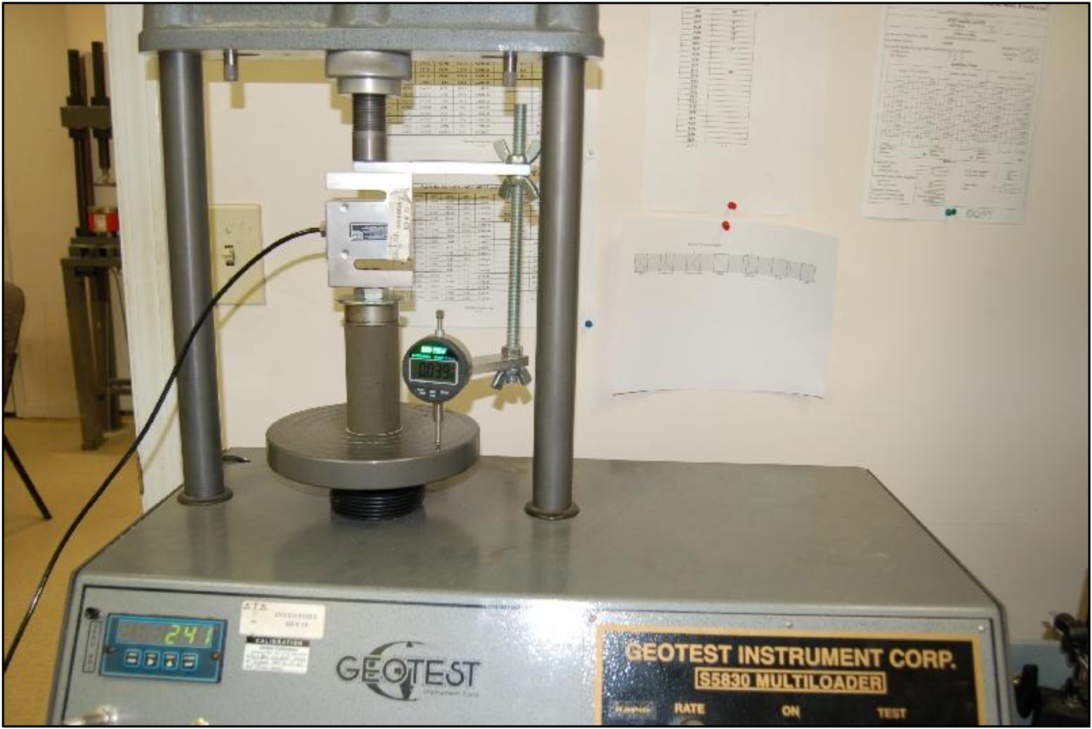
UCS is one of the most basic parameters of rock strength, and the most common determination performed for bore ability predictions. It is measured in accordance with the procedures given in ASTM D2938, with the length to diameter ratio of 2 by using NX-size core samples. 3 to 5 UCS determinations are recommended to achieve statistical significance of the results. If the sample length to diameter ratio was greater or less than 2, ASTM recommends a correction factor that is applied to the UCS value determined from testing. UCS measurements are made using an electronic-servo controlled MTS stiff testing machine with a capacity of 220 kips. Loading data and other test parameters are recorded with a computer based data acquisition system, and the data is subsequently reduced and analyzed with a customized spreadsheet program.

The most important test for rock in the field of dredging is the uniaxial unconfined compressive strength (UCS). In the test a cylindrical rock sample is axial loaded till failure. Except the force needed, the deformation is measured too. So the complete stress-strain curve is measured from which the deformation modulus and the specific work of failure can be calculated. The unconfined compressive strength of the specimen is calculated by dividing the maximum load at failure by the sample cross-sectional area:

\[\ \sigma_{\mathrm{c}}=\frac{\mathrm{F}}{\mathrm{A}}\tag{2-29}\]

Figure 2-24: A UCS test facility (Timely Engineering Soil Tests, LLC).

Figure 2-25: Bending (Vlasblom (2003-2007)).

2.4.9. Unconfined Tensile Strength

The uniaxial unconfined tensile strength is defined in the same way as the compressive strength. Sample preparation and testing procedure require much effort and not commonly done. Another method to determine the tensile strength, also commonly not used, is by bending a sample.

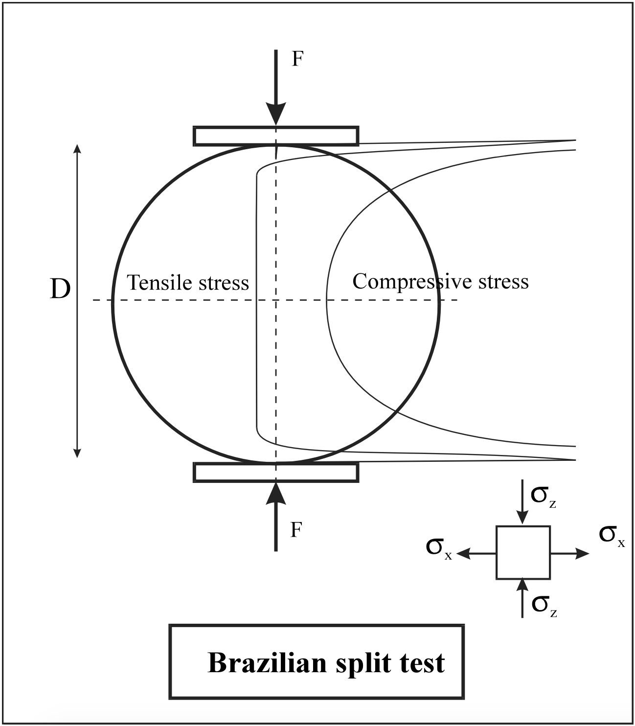
2.4.10. BTS or Brazilian Tensile Strength

Indirect, or Brazilian, tensile strength is measured using NX-size core samples cut to an approximate 0.5 length- to-diameter ratio, and following the procedures of ASTM D3967. BTS measurements are made using an electronic-servo controlled MTS stiff testing machine with a capacity of 220 kips. Loading data and other test parameters are recorded with a computer based data acquisition system, and the data is subsequently reduced and analyzed with a customized spreadsheet program. BTS provides a measure of rock toughness, as well as strength. The indirect tensile strength is calculated as follows (Fairhurst (1964)):

\[\ \sigma_{\mathrm{T}}=\frac{2 \cdot \mathrm{F}}{\pi \cdot \mathrm{L} \cdot \mathrm{D}}\tag{2-30}\]

In bedded/foliated rocks, particular attention needs to be given to loading direction with respect to bedding/foliation. The rock should be loaded so that breakage occurs in approximately the same direction as fracture propagation between adjacent cuts on the tunnel face. This is very important assessment in mechanical excavation by tunnel boring machines. The most common used test to estimate, in an indirect way, the tensile strength is the Brazilian split test. Here the cylindrical sample is tested radial.

The validity of BTS to determine de UTS is discussed by many researchers. In general it can be stated that the BTS over estimates the UTS. According to Pells (1993) this discussion is in most applications in practice largely academic.

Figure 2-26: The Brazilian split test (Vlasblom (2003-2007)).

2.4.11. Hardness

Hardness is a loosely defined term, referring the resistance to rock or minerals against an attacking tool. Hardness is determined using rebound tests (f.i. Schmidt hammer), indentation tests, (Brinell, Rockwell) or scratch tests (Mohs). The last test is based on the fact that a mineral higher in the scale can scratch a mineral lower in the scale.

Although this scale was established in the early of the 19^th century it appeared that the increment of Mohs scale corresponded with a 60% increase in indentation hardness.

Table 2-13: The Mohs scale (source Wikipedia).

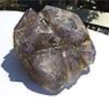
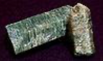
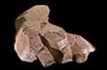
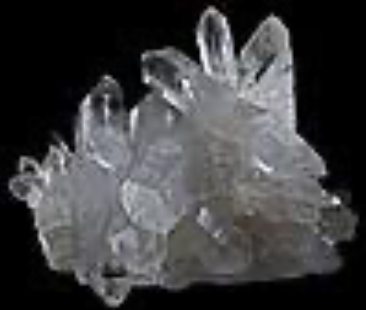
Mohs hardness	Mineral	Chemical formula	Absolute hardness.	Image
1	Talc	Mg3Si4O10(OH)2	1
2	Gypsum	CaSO4·2H2O	3
3	Calcite	CaCO3	9
4	Fluorite	CaF2	21
5	Apatite	Ca5(PO4)3(OH^−,Cl^−,F^−)	48
6	Orthoclase	KAlSi3O8	72
7	Quartz	SiO2	100
8	Topaz	Al2SiO4(OH^−,F^−)2	200
9	Corundum	Al2O3	400
10	Diamond	C	1600