6.9: Determination of the Shear Angle β

The equations are derived with which the forces on a straight blade can be determined according to the method of Coulomb (see Verruyt (1983)). Unknown in these equations is the shear angle β. In literature several methods are used to determine this shear angle.
The oldest is perhaps the method of Coulomb (see Verruyt (1983)). This method is widely used in sheet pile wall calculations. Since passive earth pressure is the cause for failure here, it is necessary to find the shear angle at which the total, on the earth, exerted force by the sheet pile wall is at a minimum.

When the water pressures are not taken into account, an analytical solution for this problem can be found. Another failure criterion is used by Hettiaratchi and Reece (1966), (1967A), (1967B), (1974) and (1975). This principle is based upon the cutting of dry sand. The shear plane is not assumed to be straight as in the method of Coulomb, but the shear plane is composed of a logarithmic spiral from the blade tip that changes into a straight shear plane under an angle of 45^o - φ/2 with the horizontal to the sand surface. The straight part of the shear plane is part of the so-called passive Rankine zone. The origin of the logarithmic spiral is chosen such that the total force on the blade is minimal.

There are perhaps other failure criterions for sheet pile wall calculations known in literature, but these mechanisms are only suited for a one-time failure of the earth. In the cutting of soil the process of building up stresses and next the collapse of the earth is a continuous process.

Another criterion for the collapse of earth is the determination of those failure conditions for which the total required strain energy is minimal. Rowe (1962) and Josselin de Jong (1976) use this principle for the determination of the angle under which local shear takes place. From this point of view it seems plausible to assume that those failure criterions for the cutting of sand have to be chosen, for which the cutting work is minimal. This implies that the shear angle β has to be chosen for which the cutting work and therefore the horizontal force, exerted by the blade on the soil, is minimal. Miedema (1985B) and (1986B) and Steeghs (1985A) and (1985B) have chosen this method.

Assuming that the water pressures are dominant in the cutting of packed water saturated sand, and thus neglecting adhesion, cohesion, gravity, inertia forces, flow resistance and under-pressure behind the blade, the force F_h (equation (6-14)) becomes for the non-cavitating situation:

\[\ \mathrm{F_h}=\left(\begin{array}{left}-\mathrm{p}_{2 \mathrm{m}} \cdot \mathrm{h}_{\mathrm{b}} \cdot \frac{\sin (\alpha)}{\sin (\alpha)}\\
+\mathrm{p}_{\mathrm{2} \mathrm{m}} \cdot \mathrm{h}_{\mathrm{b}} \cdot \frac{\sin (\alpha+\beta+\varphi) \cdot \sin (\alpha+\delta)}{\sin (\alpha+\beta+\delta+\varphi) \cdot \sin (\alpha)}\\
+\mathrm{p}_{1 \mathrm{m}} \cdot \mathrm{h}_{\mathrm{i}} \cdot \frac{\sin (\varphi) \cdot \sin (\alpha+\delta)}{\sin (\alpha+\beta+\delta+\varphi) \cdot \sin (\beta)}\end{array}\right)\cdot \mathrm{\frac{\rho_w \cdot g \cdot v_c \cdot \varepsilon\cdot h_i \cdot w}{(a_1 \cdot k_i + a_2 \cdot k_{max})}}\tag{6-60}\]

With the following simplification:

\[\ \mathrm{F}_{\mathrm{h}}^{\prime}=\frac{\mathrm{F}_{\mathrm{h}}}{\frac{\rho_{\mathrm{w}} \cdot \mathrm{g} \cdot \mathrm{v}_{\mathrm{c}} \cdot \varepsilon \cdot \mathrm{h}_{\mathrm{i}} \cdot \mathrm{w}}{\left(\mathrm{a}_{1} \cdot \mathrm{k}_{\mathrm{i}}+\mathrm{a}_{2} \cdot \mathrm{k}_{\mathrm{m a x}}\right)}}\tag{6-61}\]

Since the value of the shear angle β, for which the horizontal force is minimal, has to be found, equations (6-62) and (6-65) are set equal to zero. It is clear that this problem has to be solved iterative, because an analytical solution is impossible.

The Newton-Rhapson method works very well for this problem. In Miedema (1987 September) and 0 and 0 the resulting shear angles β, calculated with this method, can be found for several values of δ, φ, α, several ratios of h_b/h_i and for the non-cavitating and cavitating cutting process.

Figure 6-25: The forces F_h and F_t as function of the shear angle β and the blade angle β.

Interesting are now the results if another method is used. To check this, the shear angles have also been determined according Coulomb’s criterion: there is failure at the shear angle for which the total force, exerted by the blade on the soil, is minimal. The maximum deviation of these shear angles with the shear angles according Miedema (1987 September) has a value of only 3^o at a blade angle of 15^o. The average deviation is approximately 1.5^o for blade angles up to 60^o.

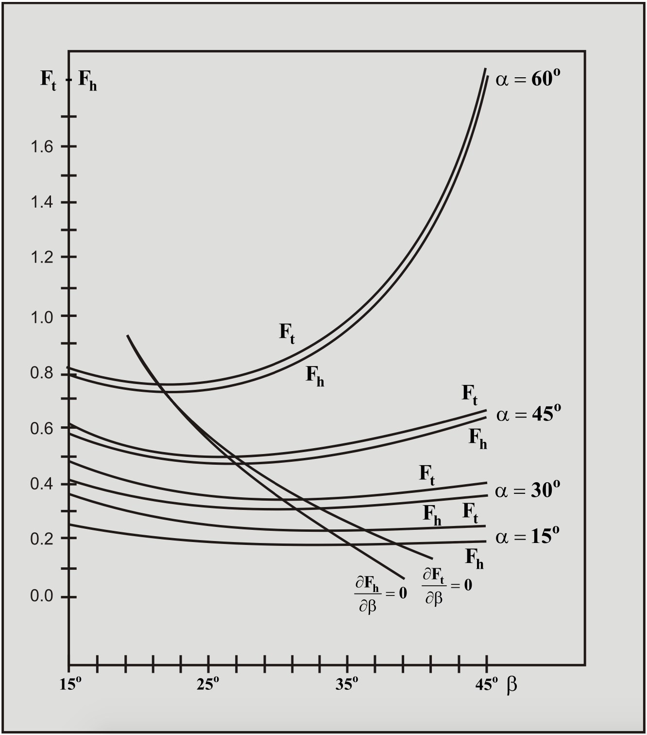
The forces have a maximum deviation of less than 1%. It can therefore be concluded that it does not matter if the total force, exerted by the soil on the blade, is minimized, or the horizontal force. Next these calculations showed that the cutting forces, as a function of the shear angle, vary only slightly with the shear angles, found using the above equation. This sensitivity increases with an increasing blade angle. Figure 6-25 shows this for the following conditions:

The forces are determined by minimizing the specific cutting energy and minimizing the total cutting force Ft. (α = 15°, 30°, 45° and 60°, δ = 24°, φ = 42°, h_b/h_i = 1 and a non-cavitating cutting process).

The derivative of the force F’_h to the shear angle β becomes:

\[\ \begin{array}{left} \frac{\partial \mathrm{F}_{\mathrm{h}}^{\prime}}{\partial \beta}=&-\mathrm{p}_{1 \mathrm{m}} \cdot \mathrm{h}_{\mathrm{i}} \cdot \frac{\sin (\varphi) \cdot \sin (\alpha+2 \cdot \beta+\delta+\varphi) \cdot \sin (\alpha+\delta)}{\sin ^{2}(\beta) \cdot \sin (\alpha+\beta+\delta+\varphi)^{2}} & \\&+\mathrm{p}_{2 \mathrm{m}} \cdot \mathrm{h}_{\mathrm{b}} \cdot \frac{\sin (\delta) \cdot \sin (\alpha+\delta)}{\sin (\alpha) \cdot \sin (\alpha+\beta+\delta+\varphi)^{2}} & \\&+\frac{\partial \mathrm{p}_{1 \mathrm{m}}}{\partial \beta} \cdot \mathrm{h}_{\mathrm{i}} \cdot \frac{\sin (\varphi) \cdot \sin (\alpha+\delta)}{\sin (\beta) \cdot \sin (\alpha+\beta+\delta+\varphi)} & \\&+\frac{\partial \mathrm{p}_{2 \mathrm{m}}}{\partial \beta} \cdot \mathrm{h}_{\mathrm{b}} \cdot\left\{\frac{\sin (\alpha+\beta+\varphi) \cdot \sin (\alpha+\delta)}{\sin (\alpha) \cdot \sin (\alpha+\beta+\delta+\varphi)}-1\right\}=\mathrm{0} \end{array}\tag{6-62}\]

For the cavitating situation this gives for the force F_h:

\[\ \mathrm{F_h}=\left(\begin{array}{left} -\mathrm{h}_{\mathrm{b}} \cdot \frac{\sin (\alpha)}{\sin (\alpha)}+\mathrm{h}_{\mathrm{b}} \cdot \frac{\sin (\alpha+\beta+\varphi) \cdot \sin (\alpha+\delta)}{\sin (\alpha+\beta+\delta+\varphi) \cdot \sin (\alpha)}\\
+\mathrm{h}_{\mathrm{i}} \cdot \frac{\sin (\varphi) \cdot \sin (\alpha+\delta)}{\sin (\alpha+\beta+\delta+\varphi) \cdot \sin (\beta)}\end{array}\right)\cdot \mathrm{\rho_w \cdot g\cdot (z+10)\cdot w}\tag{6-63}\]

With the following simplification:

\[\ \mathrm{F}_{\mathrm{h}}^{\prime}=\frac{\mathrm{F}_{\mathrm{h}}}{\rho_{\mathrm{w}} \cdot \mathrm{g} \cdot(\mathrm{z}+\mathrm{1 0}) \cdot \mathrm{w}}\tag{6-64}\]

The derivative of the force F'_h to the shear angle β becomes:

\[\ \begin{array}{left}\frac{\partial \mathrm{F_{h}}^{\prime}}{\partial \beta}=-\mathrm{h_{i}} \cdot \frac{\sin (\varphi) \cdot \sin (\alpha+2 \cdot \beta+\delta+\varphi) \cdot \sin (\alpha+\delta)}{\sin ^{2}(\beta) \cdot \sin (\alpha+\beta+\delta+\varphi)^{2}}\\
+\mathrm{h_{b}} \cdot \frac{\sin (\delta) \cdot \sin (\alpha+\delta)}{\sin (\alpha) \cdot \sin (\alpha+\beta+\delta+\varphi)^{2}}=0\end{array}\tag{6-65}\]

For the cavitating cutting process equation (6-65) can be simplified to:

\[\ \mathrm{h}_{\mathrm{b}} \cdot \sin (\delta) \cdot \sin ^{2}(\beta)=\mathrm{h}_{\mathrm{i}} \cdot \sin (\alpha) \cdot \sin (\phi) \cdot \sin (\alpha+2 \cdot \beta+\delta+\varphi)\tag{6-66}\]

The iterative results can be approximated by:

\[\ \beta=61.29^{\circ}+0.345 \cdot \mathrm{\frac{h_{b}}{h_{i}}}-0.3068 \cdot \alpha-0.4736 \cdot \delta-0.248 \cdot \varphi\tag{6-67}\]