7.3: The Influence of Strain Rate on the Cutting Process

7.3.1. Introduction

Previous researchers, especially Mitchell (1976), have derived equations for the strain rate dependency of the cohesion based on the "rate process theory". However the resulting equations did not allow pure cohesion and adhesion. In many cases the equations derived resulted in a yield stress of zero or minus infinity for a material at rest. Also empirical equations have been derived giving the same problems.

Based on the "rate process theory" with an adapted Boltzman probability distribution, the Mohr-Coulomb failure criteria will be derived in a form containing the influence of the deformation rate on the parameters involved. The equation derived allows a yield stress for a material at rest and does not contradict the existing equations, but confirms measurements of previous researchers. The equation derived can be used for silt and for clay, giving both materials the same physical background. Based on the equilibrium of forces on the chip of soil cut, as derived by Miedema (1987 September) for soil in general, criteria are formulated to predict the failure mechanism when cutting clay. A third failure mechanism can be distinguished, the "curling type". Combining the equation for the deformation rate dependency of cohesion and adhesion with the derived cutting equations, allows the prediction of the failure mechanism and the cutting forces involved. The theory developed has been verified by using data obtained by Hatamura and Chijiiwa (1975), (1976A), (1976B), (1977A) and (1977B) with respect to the adapted rate process theory and data obtained by Stam (1983) with respect to the cutting forces. However since the theory developed confirms the work carried out by previous researchers its validity has been proven in advance. In this chapter simplifications have been applied to allow a clear description of the phenomena involved.

The theory in this chapter has been published by Miedema (1992) and later by Miedema (2009) and (2010).

Figure 7-5: The Boltzman probability distribution.

Figure 7-6: The probability of exceeding an energy level Ea.

7.3.2. The Rate Process Theory

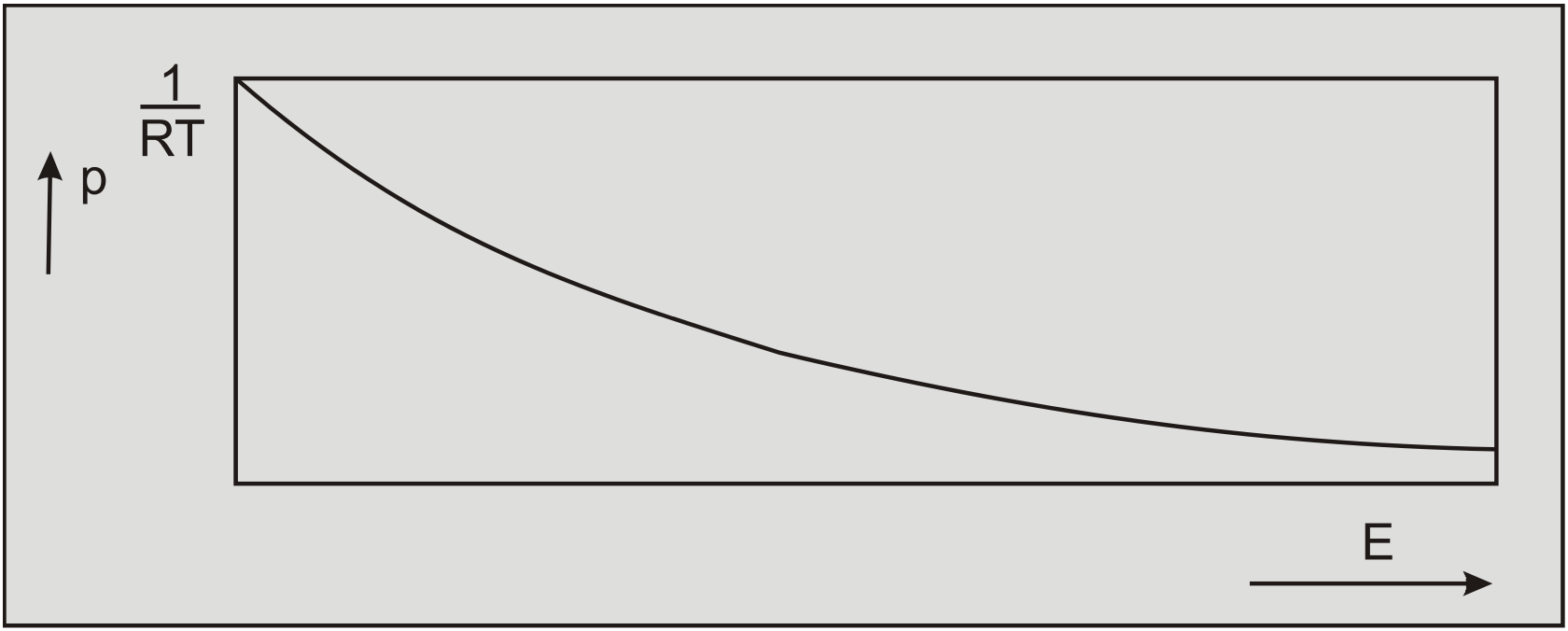
It has been noticed by many researchers that the cohesion and adhesion of clay increase with an increasing deformation rate. It has also been noticed that the failure mechanism of clay can be of the "flow type" or the "tear type", similar to the mechanisms that occur in steel cutting. The rate process theory can be used to describe the phenomena occurring in the processes involved. This theory, developed by Glasstone, Laidler and Eyring (1941) for the modeling of absolute reaction rates, has been made applicable to soil mechanics by Mitchell (1976). Although there is no physical evidence of the validity of this theory it has proved valuable for the modeling of many processes such as chemical reactions. The rate process theory, however, does not allow strain rate independent stresses such as real cohesion and adhesion. This connects with the starting point of the rate process theory that the probability of atoms, molecules or particles, termed flow units having a certain thermal vibration energy is in accordance with the Boltzman distribution (Figure 7-5):

\[\ \mathrm{p}(\mathrm{E})=\frac{1}{\mathrm{R} \cdot \mathrm{T}} \cdot \exp \left(\frac{-\mathrm{E}}{\mathrm{R} \cdot \mathrm{T}}\right)\tag{7-2}\]

Figure 7-7: The probability of net activation in direction of force.

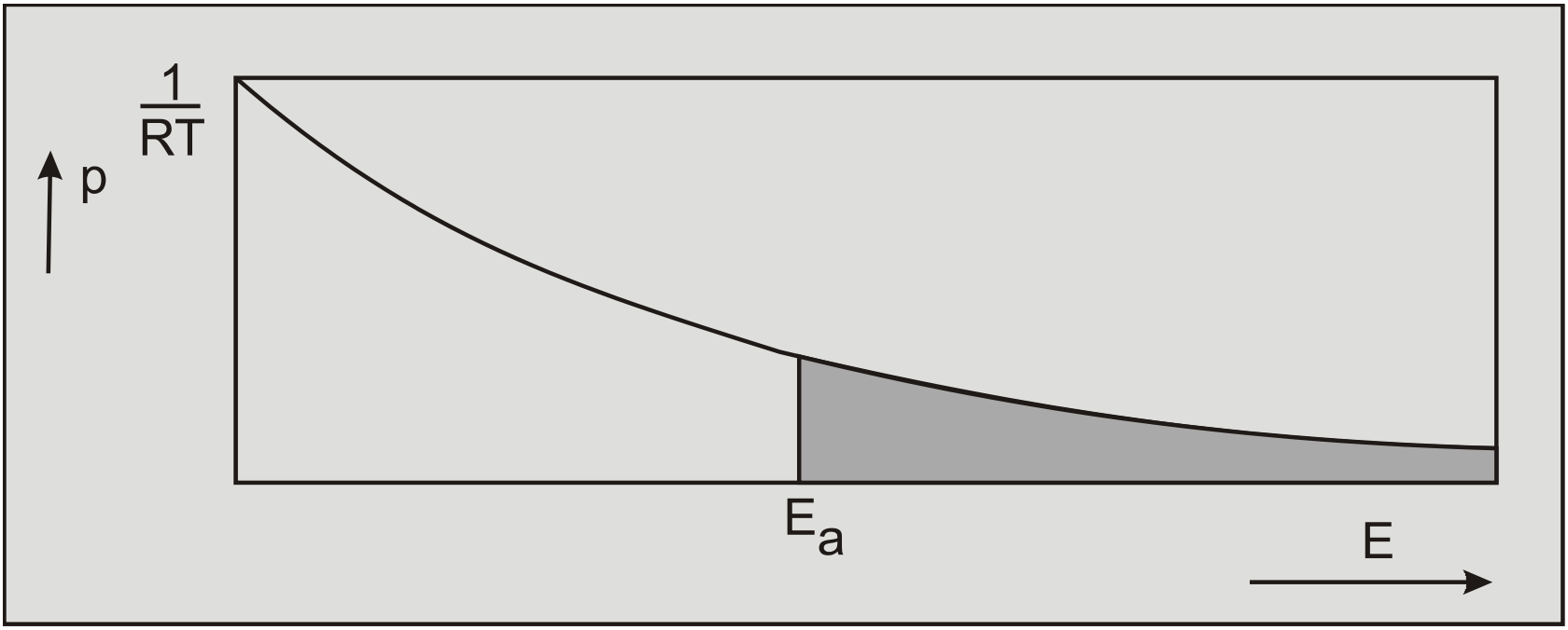
The movement of flow units participating in a time dependent flow is constrained by energy barriers separating adjacent equilibrium positions. To cross such an energy barrier, a flow unit should have an energy level exceeding certain activation energy E_a. The probability of a flow unit having an energy level greater than a certain energy level E_a can be calculated by integrating the Boltzman distribution from the energy level E_a to infinity, as depicted in Figure 7-6, this gives:

\[\ \mathrm{p}_{\mathrm{E}>\mathrm{E}_{\mathrm{a}}}=\exp \left(\frac{-\mathrm{E}_{\mathrm{a}}}{\mathrm{R} \cdot \mathrm{T}}\right)\tag{7-3}\]

The value of the activation energy E_a depends on the type of material and the process involved. Since thermal vibrations occur at a frequency given by kT/h, the frequency of activation of crossing energy barriers is:

\[\ v=\frac{\mathrm{k} \cdot \mathrm{T}}{\mathrm{h}} \cdot \exp \left(\frac{-\mathrm{E}_{\mathrm{a}}}{\mathrm{R} \cdot \mathrm{T}}\right)\tag{7-4}\]

In a material at rest the barriers are crossed with equal frequency in all directions. If however a material is subjected to an external force resulting in directional potentials on the flow units, the barrier height in the direction of the force is reduced by (f•λ/2) and raised by the same amount in the opposite direction. Where f represents the force acting on a flow unit and λ represents the distance between two successive equilibrium positions. From this it can be derived that the net frequency of activation in the direction of the force f is as illustrated in Figure 7-7:

\[\ v=\frac{\mathrm{k} \cdot \mathrm{T}}{\mathrm{h}} \cdot \exp \left(\frac{-\mathrm{E}_{\mathrm{a}}}{\mathrm{R} \cdot \mathrm{T}}\right) \cdot\left\{\exp \left(\frac{+\mathrm{f} \cdot \lambda}{\mathrm{2} \cdot \mathrm{k} \cdot \mathrm{T}}\right)-\exp \left(\frac{-\mathrm{f} \cdot \lambda}{\mathrm{2} \cdot \mathrm{k} \cdot \mathrm{T}}\right)\right\}\tag{7-5}\]

If a shear stress \(\ \tau\) is distributed uniformly along S bonds between flow units per unit area then f=\(\ \tau\) /S and if the strain rate is a function X of the proportion of successful barrier crossings and the displacement per crossing according to dε/dt=X·\(\ v\) then:

\[\ \dot{\varepsilon}=2 \cdot \mathrm{X} \cdot \frac{\mathrm{k} \cdot \mathrm{T}}{\mathrm{h}} \cdot \exp \left(\frac{-\mathrm{E}_{\mathrm{a}}}{\mathrm{R} \cdot \mathrm{T}}\right) \cdot \sinh \left(\frac{\tau \cdot \lambda \cdot \mathrm{N}}{\mathrm{2} \cdot \mathrm{S} \cdot \mathrm{R} \cdot \mathrm{T}}\right) \quad \quad \mathrm{w} \mathrm{i} \mathrm{th}: \mathrm{R}=\mathrm{N} \cdot \mathrm{k}\tag{7-6}\]

From this equation, simplified equations can be derived to obtain dashpot coefficients for theological models, to obtain functional forms for the influences of different factors on strength and deformation rate, and to study deformation mechanisms in soils. For example:

\[\ \text{if } \left(\frac{\tau \cdot \lambda \cdot \mathrm{N}}{2 \cdot \mathrm{S} \cdot \mathrm{R} \cdot \mathrm{T}}\right)<1\quad\text{ then }\quad\sinh \left(\frac{\tau \cdot \lambda \cdot \mathrm{N}}{2 \cdot \mathrm{S} \cdot \mathrm{R} \cdot \mathrm{T}}\right) \approx\left(\frac{\tau \cdot \lambda \cdot \mathrm{N}}{2 \cdot \mathrm{S} \cdot \mathrm{R} \cdot \mathrm{T}}\right)\tag{7-7}\]

Resulting in the mathematical description of a Newtonian fluid flow, and:

\[\text{if } \left(\frac{\tau \cdot \lambda \cdot \mathrm{N}}{2 \cdot \mathrm{S} \cdot \mathrm{R} \cdot \mathrm{T}}\right)>\mathrm{1}\quad\text{ then }\quad\sinh \left(\frac{\tau \cdot \lambda \cdot \mathrm{N}}{\mathrm{2} \cdot \mathrm{S} \cdot \mathrm{R} \cdot \mathrm{T}}\right) \approx \frac{\mathrm{1}}{2} \cdot \exp \left(\frac{\tau \cdot \lambda \cdot \mathrm{N}}{2 \cdot \mathrm{S} \cdot \mathrm{R} \cdot \mathrm{T}}\right)\tag{7-8}\]

Resulting in a description of the Mohr-Coulomb failure criterion for soils as proposed by Mitchell et al. (1968). Zeng and Yao (1988) and (1991) used the first simplification (7-7) to derive a relation between soil shear strength and shear rate and the second simplification (7-8) to derive a relation between soil-metal friction and sliding speed.

7.3.3. Proposed Rate Process Theory

The rate process theory does not allow shear strength if the deformation rate is zero. This implies that creep will always occur since any material is always exposed to its own weight. This results from the starting point of the rate process theory, the Boltzman distribution of the probability of a flow unit exceeding a certain energy level of thermal vibration. According to the Boltzman distribution there is always a probability that a flow unit exceeds an energy level, between an energy level of zero and infinity, this is illustrated in Figure 7-6.

Since the probability of a flow unit having an infinite energy level is infinitely small, the time-span between the occurrences of flow units having an infinite energy level is also infinite, if a finite number of flow units is considered. From this it can be deduced that the probability that the energy level of a finite number of flow units does not exceed a certain limiting energy level in a finite time-span is close to 1. This validates the assumption that for a finite number of flow units in a finite time-span the energy level of a flow unit cannot exceed a certain limiting energy level E_l. The resulting adapted Boltzman distribution is illustrated in Figure 7-8. The Boltzman distribution might be a good approximation for atoms and molecules but for particles consisting of many atoms and/or molecules the distribution according to Figure 7-8 seems more reasonable, since it has never been noticed that sand grains in a layer of sand at rest, start moving because of their internal energy. In clay some movement of the clay particles seems probable since the clay particles are much smaller than the sand particles. Since particles consist of many atoms, the net vibration energy in any direction will be small, because the atoms vibrate thermally with equal frequency in all directions.

Figure 7-8: The adapted Boltzman probability distribution.

If a probability distribution according to Figure 7-8 is considered, the probability of a particle exceeding a certain activation energy E_a becomes:

\[\ \mathrm{p}_{\mathrm{E}>\mathrm{E}_{\mathrm{a}}}=\frac{\exp \left(\frac{-\mathrm{E}_{\mathrm{a}}}{\mathrm{R} \cdot \mathrm{T}}\right)-\exp \left(\frac{-\mathrm{E}_{\ell}}{\mathrm{R} \cdot \mathrm{T}}\right)}{\mathrm{1 - \operatorname { exp }}\left(\frac{-\mathrm{E}_{\ell}}{\mathrm{R} \cdot \mathrm{T}}\right)} \quad\text{ if }\quad\mathrm{E}_{\mathrm{a}}<\mathrm{E}_{\ell}\quad\text{ and }\quad\mathrm{p}_{\mathrm{E}>\mathrm{E}_{\mathrm{a}}}=\mathrm{0} \quad\text{ if }\quad\mathrm{E}_{\mathrm{a}}>\mathrm{E}_{\ell}\tag{7-9}\]

If the material is now subjected to an external shear stress, four cases can be distinguished with respect to the strain rate.

Figure 7-9: The probability of net activation in case 1.

Case 1:

The energy level \(\ \mathrm{E}_{\mathrm{a}}+\tau \lambda \mathrm{N} / 2 \mathrm{S}\) is smaller than the limiting energy level El (Figure 7-9). The strain rate equation is now: \[\ \begin{array}{left}\dot{\varepsilon}=2 \cdot \mathrm{X} \cdot \frac{\mathrm{k} \cdot \mathrm{T}}{\mathrm{h} \cdot \mathrm{i}} \cdot \exp \left(\frac{-\mathrm{E}_{\mathrm{a}}}{\mathrm{R} \cdot \mathrm{T}}\right) \cdot \sinh \left(\frac{\tau \cdot \lambda \cdot \mathrm{N}}{\mathrm{2} \cdot \mathrm{S} \cdot \mathrm{R} \cdot \mathrm{T}}\right)\\\text{with: } \mathrm{i=1-exp\left(\frac{-E_{\ell}}{R \cdot T} \right)}\end{array}\tag{7-10}\] Except for the coefficient i, necessary to ensure that the total probability remains 1, equation (7-10) is identical to equation (7-6).

Case 2:

The activation energy Ea is less than the limiting energy El, but the energy level \(\ \mathrm{E}+\tau \lambda \mathrm{N} / 2 \mathrm{S}\) is greater than the limiting energy level El (Figure 7-10). The strain rate equation is now: \[\ \dot{\varepsilon}=\mathrm{X} \cdot \frac{\mathrm{k} \cdot \mathrm{T}}{\mathrm{h} \cdot \mathrm{i}} \cdot\left\{\exp \left(-\left(\frac{\mathrm{E}_{\mathrm{a}}}{\mathrm{R} \cdot \mathrm{T}}-\frac{\tau \cdot \lambda \cdot \mathrm{N}}{\mathrm{2} \cdot \mathrm{S} \cdot \mathrm{R} \cdot \mathrm{T}}\right)\right)-\exp \left(\frac{-\mathrm{E}_{\ell}}{\mathrm{R} \cdot \mathrm{T}}\right)\right\}\tag{7-11}\]

Case 3:

The activation energy Ea is greater than the limiting energy El, but the energy level \(\ \mathrm{E}_{\mathrm{a}}-\tau \lambda \mathrm{N} / \mathrm{2} \mathrm{S}\) is less than the limiting energy level El (Figure 7-11). The strain rate equation is now:  \[\ \dot{\varepsilon}=\mathrm{X} \cdot \frac{\mathrm{k} \cdot \mathrm{T}}{\mathrm{h} \cdot \mathrm{i}} \cdot\left\{\exp \left(-\left(\frac{\mathrm{E}_{\mathrm{a}}}{\mathrm{R} \cdot \mathrm{T}}-\frac{\tau \cdot \lambda \cdot \mathrm{N}}{\mathrm{2} \cdot \mathrm{S} \cdot \mathrm{R} \cdot \mathrm{T}}\right)\right)-\exp \left(\frac{-\mathrm{E}_{\ell}}{\mathrm{R} \cdot \mathrm{T}}\right)\right\}\tag{7-12}\] Equation (7-12) appears to be identical to equation (7-11), but the boundary conditions differ.

Case 4:

The activation energy Ea is greater than the limiting energy El and the energy level \(\ \mathrm{E}_{\mathrm{a}}-\tau \lambda \mathrm{N} / \mathrm{2} \mathrm{S}\) is greater than the limiting energy level El (Figure 7-12). The strain rate will be equal to zero in this case.

The cases 1 and 2 are similar to the case considered by Mitchell (1976) and still do not permit true cohesion and adhesion. Case 4 considers particles at rest without changing position within the particle matrix. Case 3 considers a material on which an external shear stress of certain magnitude must be applied to allow the particles to cross energy barriers, resulting in a yield stress (true cohesion or adhesion).

Figure 7-10: The probability of net activation in case 2.

Figure 7-11: The probability of net activation in case 3.

Figure 7-12: The probability of net activation in case 4.

From equation (7-12) the following equation for the shear stress can be derived:

\[\ \begin{array}{left}\tau=\left(\mathrm{E}_{\mathrm{a}}-\mathrm{E}_{\ell}\right) \cdot \frac{\mathrm{2} \cdot \mathrm{S}}{\lambda \cdot \mathrm{N}}+\mathrm{R} \cdot \mathrm{T} \cdot \frac{\mathrm{2} \cdot \mathrm{S}}{\lambda \cdot \mathrm{N}} \cdot \ln \left(\mathrm{1}+\frac{\dot{\varepsilon}}{\dot{\varepsilon}_{\mathrm{0}}}\right)\\
\text{with: }\dot{\varepsilon}_{\mathrm{0}}=\frac{\mathrm{X} \cdot \mathrm{k} \cdot \mathrm{T}}{\mathrm{h} \cdot \mathrm{i}} \cdot \exp \left(\frac{-\mathrm{E}_{\ell}}{\mathrm{R} \cdot \mathrm{T}}\right)\end{array}\tag{7-13}\]

According to Mitchell (1976), if no shattering of particles occurs, the relation between the number of bonds S and the effective stress σ_e can be described by the following equation:

\[\ \mathrm{S}=\mathrm{a}+\mathrm{b} \cdot \sigma_{\mathrm{e}}\tag{7-14}\]

Lobanov and Joanknecht (1980) confirmed this relation implicitly for pressures up to 10 bars for clay and paraffin wax. At very high pressures they found an exponential relation that might be caused by internal failure of the particles. For the friction between soil and metal Zeng and Yao (1988) also used equation (7-14), but for the internal friction Zeng and Yao (1991) used a logarithmic relationship, which contradicts Lobanov and Joanknecht and Mitchell, although it can be shown by Taylor series approximation that a logarithmic relation can be transformed into a linear relation for values of the argument of the logarithm close to 1. Since equation (7-14) contains the effective stress it is necessary that the clay used, is fully consolidated. Substituting equation (7-14) in equation (7-13) gives:

\[\ \begin{array}{left} \tau=& \mathrm{a} \cdot\left\{\left(\mathrm{E}_{\mathrm{a}}-\mathrm{E}_{\ell}\right) \cdot \frac{\mathrm{2}}{\lambda \cdot \mathrm{N}}+\mathrm{R} \cdot \mathrm{T} \cdot \frac{\mathrm{2}}{\lambda \cdot \mathrm{N}} \cdot \ln \left(\mathrm{1}+\frac{\dot{\varepsilon}}{\dot{\varepsilon}_{0}}\right)\right\} \\ &+\mathrm{b} \cdot\left\{\left(\mathrm{E}_{\mathrm{a}}-\mathrm{E}_{\ell}\right) \cdot \frac{\mathrm{2}}{\lambda \cdot \mathrm{N}}+\mathrm{R} \cdot \mathrm{T} \cdot \frac{2}{\lambda \cdot \mathrm{N}} \cdot \ln \left(\mathrm{1}+\frac{\dot{\varepsilon}}{\dot{\varepsilon}_{0}}\right)\right\} \cdot \sigma_{\mathrm{e}} \end{array}\tag{7-15}\]

Equation (7-15) is of the same form as the Mohr-Coulomb failure criterion:

\[\ \tau=\tau_{\mathrm{c}}+\sigma_{\mathrm{e}} \cdot \tan (\varphi)\tag{7-16}\]

Equation (7-15), however, allows the strain rate to become zero, which is not possible in the equation derived by Mitchell (1976). The Mitchell equation and also the equations derived by Zeng and Yao (1988) and (1991) will result in a negative shear strength at small strain rates.

7.3.4. The Proposed Theory versus some other Theories

The proposed new theory is in essence similar to the theory developed by Mitchell (1976) which was based on the "rate process theory" as proposed by Eyring (1941). It was, however, necessary to use simplifications to obtain the equation in a useful form. The following formulation for the shear stress as a function of the strain rate has been derived by Mitchell by simplification of equation (7-6):

\[\ \begin{array}{left}\tau=\mathrm{a} \cdot\left\{\mathrm{E}_{\mathrm{a}} \cdot \frac{\mathrm{2}}{\lambda \cdot \mathrm{N}}+\mathrm{R} \cdot \mathrm{T} \cdot \frac{\mathrm{2}}{\lambda \cdot \mathrm{N}} \cdot \ln \left(\frac{\dot{\varepsilon}}{\mathrm{B}}\right)\right\}\\
+\mathrm{b} \cdot\left\{\mathrm{E}_{\mathrm{a}} \cdot \frac{\mathrm{2}}{\lambda \cdot \mathrm{N}}+\mathrm{R} \cdot \mathrm{T} \cdot \frac{2}{\lambda \cdot \mathrm{N}} \cdot \ln \left(\frac{\dot{\varepsilon}}{\mathrm{B}}\right)\right\} \cdot \sigma_{\mathrm{e}}\\
\text{with: }\mathrm{B}=\frac{\mathrm{X} \cdot \mathrm{k} \cdot \mathrm{T}}{\mathrm{h}}\end{array}\tag{7-17}\]
This equation is not valid for very small strain rates, because this would result in a negative shear stress. It should be noted that for very high strain rates the equations (7-15) and (7-17) will have exactly the same form. Zeng and Yao (1991) derived the following equation by simplification of equation (7-6) and by adding some empirical elements:

\[\ \begin{array}\ln (\tau)=\mathrm{C_{1}+C_{2} \cdot \ln (\dot{\varepsilon})+C_{3} \cdot \ln \left(1+C_{4} \cdot \sigma_{e}\right)}\end{array}\tag{7-18}\]

Rewriting equation (7-18) in a more explicit form gives:

\[\ \tau=\exp \left(\mathrm{C}_{1}\right) \cdot(\dot{\varepsilon})^{\mathrm{C}_{2}} \cdot\left(1+\mathrm{C}_{4} \cdot \sigma_{\mathrm{e}}\right)^{\mathrm{C}_{3}}\tag{7-19}\]

Equation (7-19) is valid for strain rates down to zero, but not for a yield stress. With respect to the strain rate, equation (7-19) is the equation of a fluid behaving according to the power law named "power law fluids". It should be noted however that equation (7-19) cannot be derived from equation (7-6) directly and thus should be considered as an empirical equation. If the coefficient C₃ equals 1, the relation between shear stress and effective stress is similar to the relation found by Mitchell (1976). For the friction between the soil (clay and loam) and metal Zeng and Yao (1988) derived the following equation by simplification of equation (7-6):

\[\ \tau_{\mathrm{b}}=\tau_{\mathrm{y a}}+\mathrm{C}_{\mathrm{5}} \cdot \ln (\dot{\varepsilon})+\sigma_{\mathrm{e}} \cdot \tan (\delta)=\tau_{\mathrm{a}}+\sigma_{\mathrm{e}} \cdot \tan (\delta)\tag{7-20}\]

Equation (7-20) allows a yield stress, but does not allow the sliding velocity to become zero. An important conclusion of Yao and Zeng is that pasting soil on the metal surface slightly increases the friction meaning that the friction between soil and metal almost equals the shear strength of the soil.
The above-mentioned researchers based their theories on the rate process theory, other researchers derived empirical equations. Turnage and Freitag (1970) observed that for saturated clays the cone resistance varied with the penetration rate according to:

\[\ \mathrm{F}=\mathrm{a} . \mathrm{v}^{\mathrm{b}}\tag{7-21}\]

With values for the exponent ranging from 0.091 to 0.109 Wismer and Luth (1972B) and (1972A) confirmed this relation and found a value of 0.100 for the exponent, not only for cone penetration tests but also for the relation between the cutting forces and the cutting velocity when cutting clay with straight blades. Hatamura and Chijiiwa (1975), (1976A), (1976B), (1977A) and (1977B) also confirmed this relation for clay and loam cutting and found an exponent of 0.089.

Soydemir (1977) derived an equation similar to the Mitchell equation. From the data measured by Soydemir a relation according to equation (7-21) with an exponent of 0.101 can be derived. This confirms both the Mitchell approach and the power law approach.

7.3.5. Verification of the Theory Developed

The theory developed differs from the other theories mentioned in the previous paragraph, because the resulting equation (7-15) allows a yield strength (cohesion or adhesion). At a certain consolidation pressure level equation (7-15) can be simplified to:

\[\ \tau=\tau_{\mathrm{y}}+\tau_{0} \cdot \ln \left(1+\frac{\dot{\varepsilon}}{\dot{\varepsilon}_{0}}\right)\tag{7-22}\]

If \(\ (\mathrm{d} \varepsilon / \mathrm{d t}) /\left(\mathrm{d} \varepsilon_{0} / \mathrm{d} \mathrm{t}\right)\) << 1, equation (7-22) can be approximated by:

\[\ \tau=\tau_{\mathrm{y}}+\tau_{0} \cdot \frac{\dot{\varepsilon}}{\dot{\varepsilon}_{0}}\tag{7-23}\]

This approximation gives the formulation of a Bingham fluid. If the yield strength \(\ \tau_{\mathrm{y}}\) is zero, equation represents a Newtonian fluid. If (dε/dt)/(dε₀/dt) >> 1, equation (7-22) can be approximated by: 

\[\ \tau=\tau_{\mathrm{y}}+\tau_{0} \cdot \ln \left(\frac{\dot{\varepsilon}}{\dot{\varepsilon}_{0}}\right)\tag{7-24}\]

This approximation is similar to equation (7-17) as derived by Mitchell.

If (dε/dt)/(dε₀/dt) >> 1 and \(\ \tau-\tau_{\mathrm{y}}<<\tau_{\mathrm{y}}\), equation (7-22) can be approximated by:

\[\ \tau=\tau_{\mathrm{y}} \cdot\left(\frac{\dot{\varepsilon}}{\dot{\varepsilon}_{0}}\right)^{\tau_{0} / \tau_{\mathrm{y}}}\tag{7-25}\]

This approximation is similar to equation (7-21) as found empirically by Wismer and Luth (1972B) and many other researchers. The equation (7-15) derived in this paper, the equation (7-17) derived by Mitchell and the empirical equation (7-21) as used by many researchers have been fitted to data obtained by Hatamura and Chijiiwa (1975), (1976A), (1976B), (1977A) and (1977B). This is illustrated in Figure 7-13 with a logarithmic horizontal axis. Figure 7-14 gives an illustration with both axis logarithmic. These figures show that the data obtained by Hatamura and Chijiiwa fit well and that the above described approximations are valid.

The values used are \(\ \tau\)_y =28kPa, \(\ \tau\)₀ =4kPa and ε₀ =0.03/s.

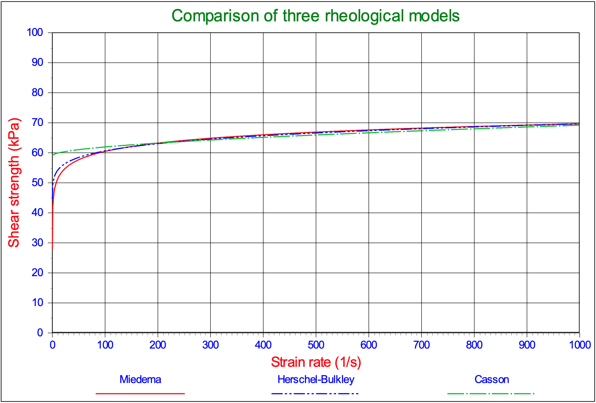
It is assumed that adhesion and cohesion can both be modeled according to equation (7-22). The research carried out by Zeng and Yao (1991) validates the assumption that this is true for adhesion. In more recent research Kelessidis et al. (2007) and (2008) utilize two rheological models, the Herschel-Bulkley model and the Casson model. The Herschel Bulkley model can be described by the following equation:

\[\ \tau=\tau_{\mathrm{y}, \mathrm{H B}}+\mathrm{K} \cdot(\dot \varepsilon)^{\mathrm{n}}\tag{7-26}\]

The Casson model can be described with the following equation:

\[\ \sqrt{\tau}=\sqrt{\tau_{\mathrm{y}, \mathrm{C a}}}+\sqrt{\mu_{\mathrm{C a}} \cdot \dot{\boldsymbol{\varepsilon}}}\tag{7-27}\]

Figure 7-15 compares these models with the model as derived in this paper. It is clear that for the high strain rates the 3 models give similar results. These high strain rates are relevant for cutting processes in dredging and offshore applications.

Figure 7-13: Shear stress as a function of strain rate with the horizontal axis logarithmic.

Figure 7-14: Shear stress as a function of strain rate with logarithmic axis.

Figure 7-15: Comparison of 3 rheological models.

7.3.6. Abelev & Valent (2010)

Abelev & Valent (2010) investigated the strain rate dependency of the strength of soft marine deposits of the Gulf of Mexico. They used a precision rheometer with rotational rates from 0.25 up to 1000 1/min and water contents of 55% to 95%. They describe several models like an inverse hyperbolic sine:

\[\ \tau=\tau_{\mathrm{y}}+\tau_{0} \cdot \arcsin \left(\frac{\dot{\varepsilon}}{\dot{\varepsilon}_{0}}\right)\tag{7-28}\]

A logarithmic law and a power law:

\[\ \tau=\tau_{\mathrm{y}}+\tau_{0} \cdot \log _{10}\left(\frac{\dot{\varepsilon}}{\dot{\varepsilon}_{0}}\right) \quad\text{ and }\quad \tau=\tau_{\mathrm{y}} \cdot\left(\frac{\dot{\varepsilon}}{\dot{\varepsilon}_{0}}\right)^{\beta}\tag{7-29}\]

Figure 7-16: Abelev & Valent (2010) data.

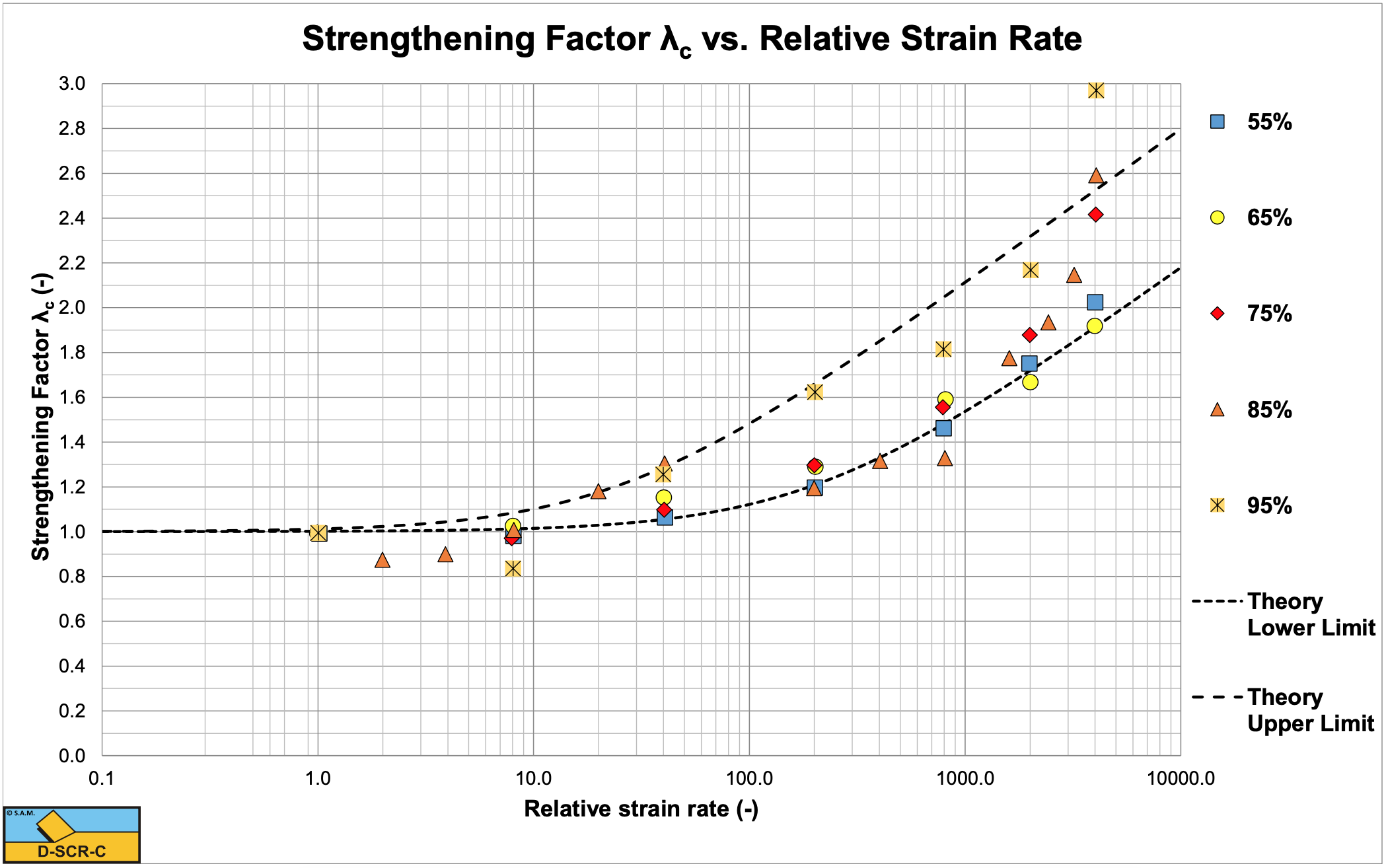
The data of Abelev & Valent (2010) are shown in Figure 7-16, together with a lower limit and an upper limit based on the equation derived in this chapter. Based on their experiments they suggest a modified power law:

\[\ \tau=\tau_{\mathrm{y}}+\tau_{0} \cdot\left(\frac{\dot{\varepsilon}}{\dot{\varepsilon}_{0}}\right)^{\beta}\tag{7-30}\]

The use of the equation derived in this chapter however gives even better results.

\[\ \tau=\tau_{\mathrm{y}}+\tau_{0} \cdot \ln \left(1+\frac{\dot{\varepsilon}}{\dot{\varepsilon}_{0}}\right)\tag{7-31}\]

One can see some dependency of the strengthening effect on the water content. It seems that the higher the water content, the larger the strengthening effect.

7.3.7. Resulting Equations for the Cutting Process

The strain rate is the rate of change of the strain with respect to time and can be defined as a velocity divided by a characteristic length. For the cutting process it is important to relate the strain rate to the cutting (deformation) velocity v_c and the layer thickness h_i. Since the deformation velocity is different for the cohesion in the shear plane and the adhesion on the blade, two different equations are found for the strain rate as a function of the cutting velocity.

\[\ \dot{\varepsilon}_{\mathrm{c}}=1.4 \cdot \frac{\mathrm{v}_{\mathrm{c}}}{\mathrm{h}_{\mathrm{i}}} \cdot \frac{\sin (\alpha)}{\sin (\alpha+\beta)}\tag{7-32}\]

\[\ \dot{\varepsilon}_{\mathrm{a}}=1.4 \cdot \frac{\mathrm{v}_{\mathrm{c}}}{\mathrm{h}_{\mathrm{i}}} \cdot \frac{\sin (\beta)}{\sin (\alpha+\beta)}\tag{7-33}\]

This results in the following two equations for the multiplication factor for cohesion (internal shear strength) and adhesion (external shear strength). With \(\ \tau_\mathrm{y}\) the cohesion at zero strain rate.

\[\ \lambda_{\mathrm{c}}=\mathrm{1 + \frac { \tau _ { 0 } } { \tau _ { \mathrm { y } } } \cdot \operatorname { ln }}\left(1+\frac{1.4 \cdot \frac{\mathrm{v}_{\mathrm{c}}}{\mathrm{h}_{\mathrm{i}}} \cdot \frac{\sin (\alpha)}{\sin (\alpha+\beta)}}{\dot{\varepsilon}_{0}}\right)\tag{7-34}\]

\[\ \lambda_{\mathrm{a}}=1+\frac{\tau_{0}}{\tau_{\mathrm{y}}} \cdot \ln \left(1+\frac{1.4 \cdot \frac{\mathrm{v}_{\mathrm{c}}}{\mathrm{h}_{\mathrm{i}}} \cdot \frac{\sin (\beta)}{\sin (\alpha+\beta)}}{\dot{\varepsilon}_{0}}\right)\tag{7-35}\]

With:

\[\ \tau_{0} / \tau_{\mathrm{y}}=\mathrm{0 .1 4 2 8}, \dot{\varepsilon}_{0}=\mathrm{0 .0 3}\tag{7-36}\]

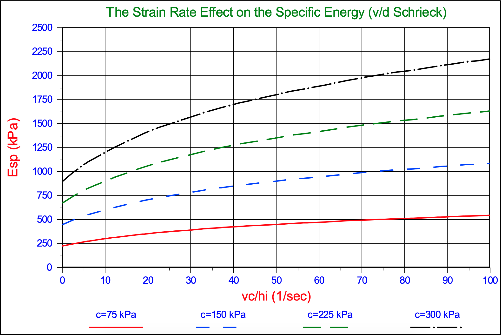
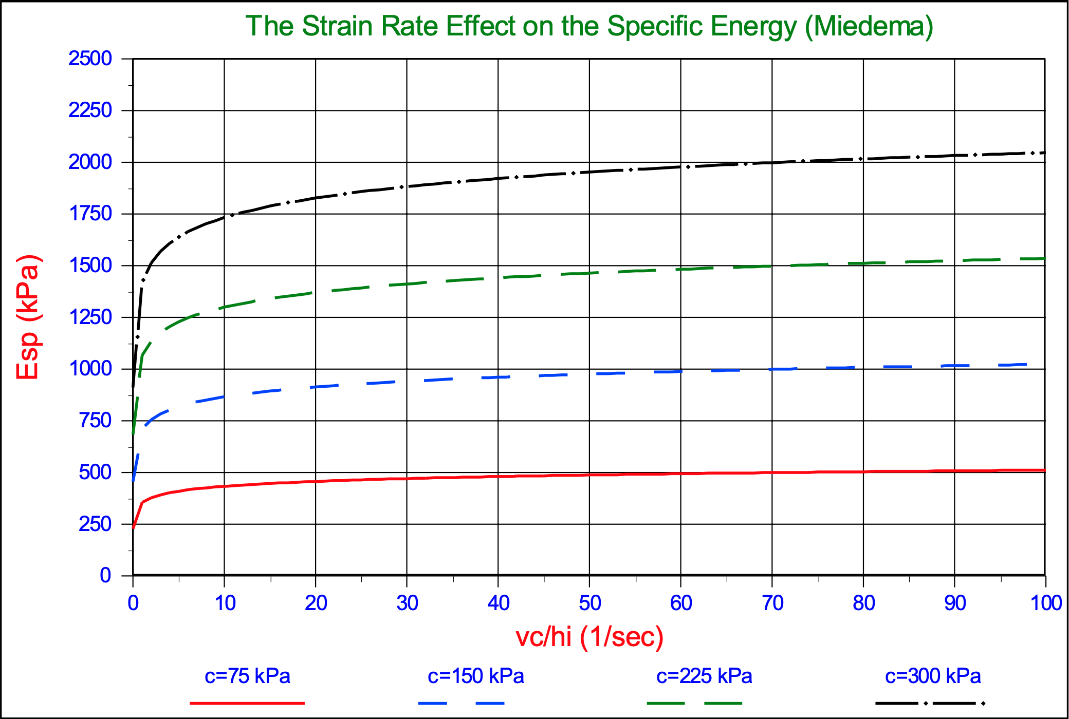
Van der Schrieck (1996) published a graph showing the effect of the deformation rate on the specific energy when cutting clay. Although the shape of the curves found are a bit different from the shape of the curves found with equations (7-34) and (7-35), the multiplication factor for, in dredging common deformation rates, is about 2. This factor matches the factor found with the above equations.

Figure 7-17: Comparison of the model developed with the v/d Schrieck (1996) model.