9.2: The Flow Type and the Crushed Type

First of all it is assumed that the hyperbaric cutting mechanism is similar to the Flow Type as is shown in Figure 9-5. There may be 3 mechanisms that might explain the influence of large hydrostatic pressures:

1. When a tensile failure occurs, water has to flow into the crack, but the formation of the crack goes so fast that cavitation will occur.

2. A second possible mechanism that might occur is an increase of the pore volume due to the elasticity of the rock and the pore water. If high tensile stresses exist in the rock, then the pore volume will increase due to elasticity. Because of the very low permeability of the rock, the compressibility of the pore water will have to deal with this. Since the pore water is not very compressible, at small volume changes this will already result in large under pressures in the pores. Whether this will lead to full cavitation of the pore water is still a question.

3. Due to the high effective grain stresses, the particles are removed from the matrix which normally keeps them together and makes it a rock. This will happen near the shear plane. The loose particles will be subject to dilatation, resulting in an increase of the pore volume. This pore volume increase results in water flow to the shear plane, which can only occur if there is an under pressure in the pores in the shear plane. If this under pressure reaches the water vapor pressure, cavitation will occur, which is the lower limit for the absolute pressures and the upper limit for the pressure difference between the bottom hole or hydrostatic pressure and the pore water pressure. The pressure difference is proportional to the cutting velocity and the dilatation, squared proportional to the layer thickness and reversely proportional to the permeability of the rock. If the rock is very impermeable, cavitation will always occur and the cutting forces will match the upper limit.

Now under atmospheric conditions, the compressive strength of the rock will be much bigger than the atmospheric pressure; usually the rock will have a compressive strength of 1 MPa or more while the atmospheric pressure is just 100 kPa. Strong rock may have compressive strengths of 10’s of MPa’s, so the atmospheric pressure and thus the effect of cavitation in the pores or the crack can be neglected. However in oil drilling and deep sea mining at water depths of 3000 m nowadays plus a few 1000’s m into the seafloor (in case of oil drilling), the hydrostatic pressure could easily increase to values higher than 10 MPa up to 100 MPa causing softer rock to behave ductile, where it would behave brittle under low hydrostatic pressures.

It should be noted that brittle-tear failure, which is tensile failure, will only occur under atmospheric conditions and small blade angles as used in dredging and mining. With blade angles larger than 90° brittle-tear will never occur (see Figure 8-38). Brittle-shear may occur in all cases under atmospheric conditions.
Now what is the difference between rock cutting under atmospheric conditions and under hyperbaric conditions? The difference is the extra pore pressure forces W₁ and W₂ on the shear plane and on the blade as will be explained next.

Figure 9-4: The definitions of the cutting process.

Figure 9-5: The Flow Type cutting mechanism.

Figure 9-6: The Crushed Type cutting mechanism.

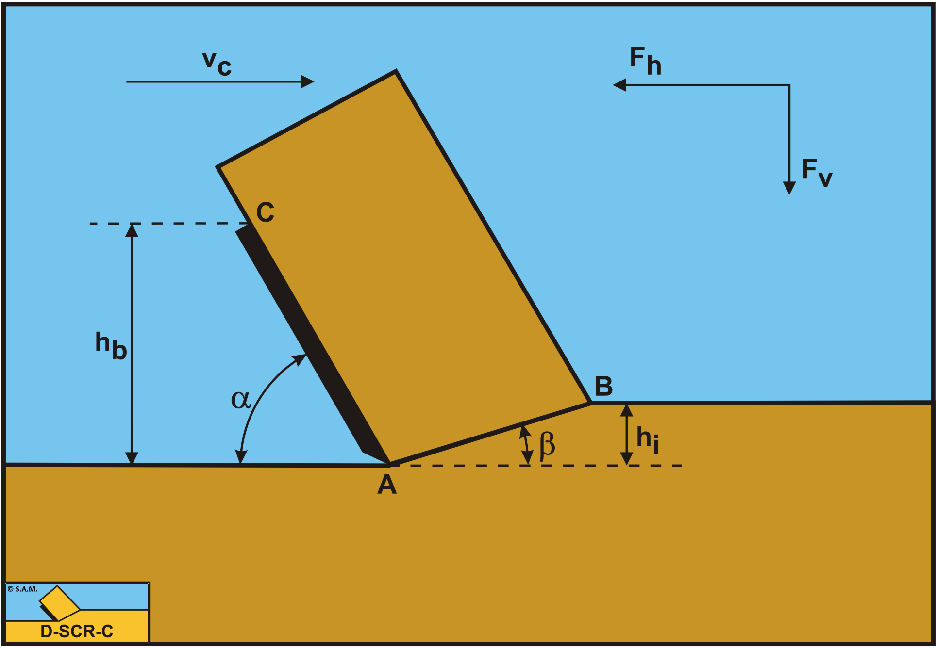
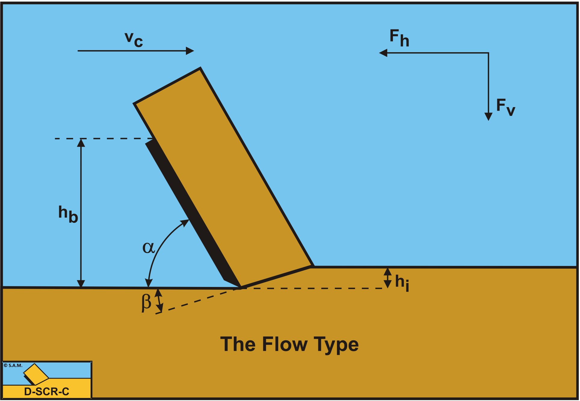
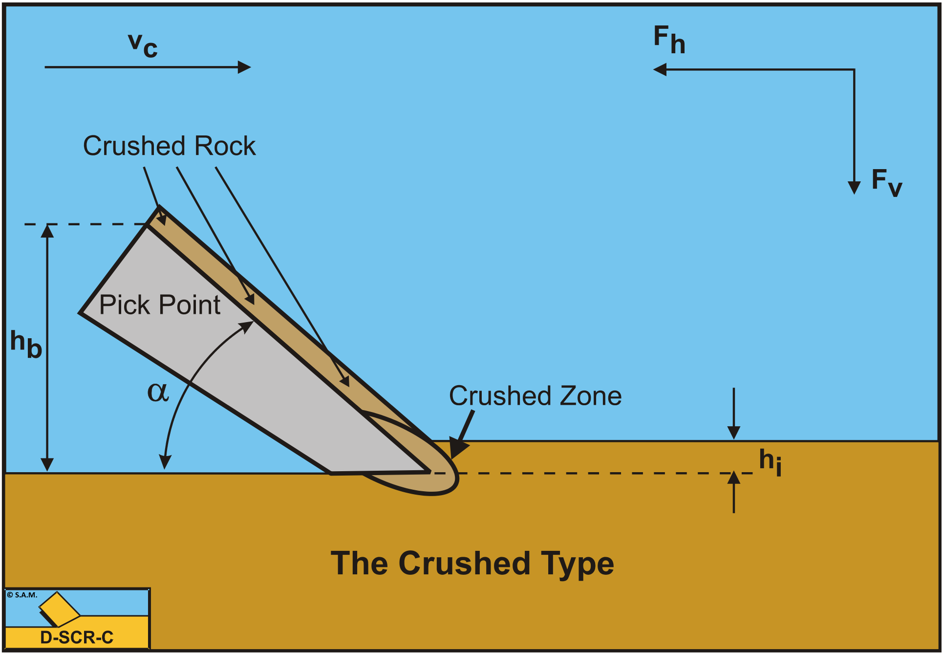
Figure 9-7 illustrates the forces on the layer of rock cut. The forces acting on this layer are:

1. A normal force acting on the shear surface N₁ resulting from the grain stresses.

2. A shear force S₁ as a result of internal friction N₁·tan(φ).

3. A force W₁ as a result of water under pressure in the shear zone.

4. A shear force C as a result of the cohesive shear strength \(\ \tau_\mathrm{c}\) or c. This force can be calculated by multiplying the cohesive shear strength \(\ \tau_\mathrm{c}\)/c with the area of the shear plane.

5. A force normal to the blade N₂ resulting from the grain stresses.

6. A shear force S₂ as a result of the external friction N₂·tan(δ).

7. A shear force A as a result of pure adhesion between the rock and the blade \(\ \tau_\mathrm{a}\) or a. This force can be calculated by multiplying the adhesive shear strength \(\ \tau_\mathrm{a}\)/a of the rock with the contact area between the rock and the blade. In most rocks this force will be absent.

8. A force W₂ as a result of water under pressure on the blade

The normal force N₁ and the shear force S₁ on the shear plane can be combined to a resulting grain force K₁.

\[\ \mathrm{K}_{1}=\sqrt{\mathrm{N}_{1}^{2}+\mathrm{S}_{1}^{2}}\tag{9-2}\]

The forces acting on a straight blade when cutting rock, can be distinguished as:

1. A force normal to the blade N₂ resulting from the grain stresses.

2. A shear force S₂ as a result of the external friction N2·tan(δ).

3. A shear force A as a result of pure adhesion between the rock and the blade \(\ \tau_\mathrm{a}\) or c. This force can be calculated  by multiplying the adhesive shear strength \(\ \tau_\mathrm{a}\)/a of the rock with the contact area between the rock and the blade. In most rocks this force will be absent.

4. A force W₂ as a result of water under pressure on the blade

Figure 9-7: The forces on the layer cut in rock (hyperbaric).

Figure 9-8: The forces on the blade in rock (hyperbaric).

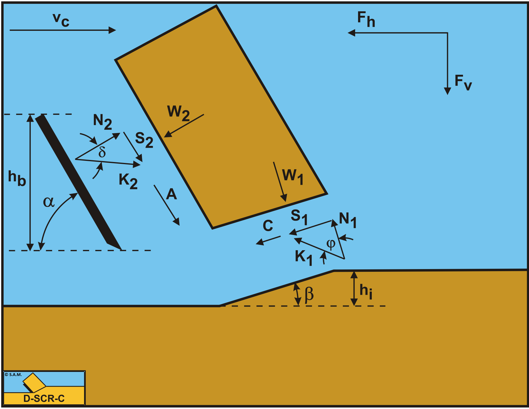
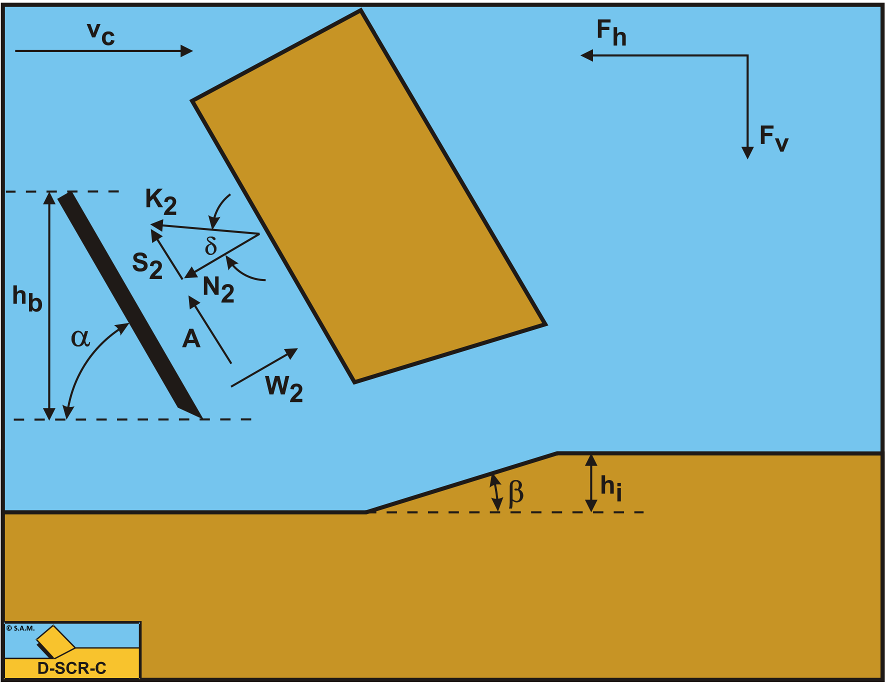
These forces are shown in Figure 9-8. If the forces N₂ and S₂ are combined to a resulting force K₂ and the adhesive force and the water under pressures are known, then the resulting force K₂ is the unknown force on the blade. By taking the horizontal and vertical equilibrium of forces an expression for the force K₂ on the blade can be derived.

\[\ \mathrm{K}_{2}=\sqrt{\mathrm{N}_{\mathrm{2}}^{\mathrm{2}}+\mathrm{S}_{\mathrm{2}}^{\mathrm{2}}}\tag{9-3}\]

The horizontal equilibrium of forces:

\[\  \sum \mathrm{F}_{\mathrm{h}}= \mathrm{K}_{1} \cdot \sin (\beta+\varphi)-\mathrm{W}_{1} \cdot \sin (\beta)+\mathrm{C} \cdot \cos (\beta) -\mathrm{A} \cdot \cos (\alpha)+\mathrm{W}_{2} \cdot \sin (\alpha)-\mathrm{K}_{2} \cdot \sin (\alpha+\delta)=0 \tag{9-4}\]

The vertical equilibrium of forces:

\[\ \sum \mathrm{F}_{\mathrm{v}}=-\mathrm{K}_{1} \cdot \cos (\beta+\varphi)+\mathrm{W}_{1} \cdot \cos (\beta)+\mathrm{C} \cdot \sin (\beta) +\mathrm{A} \cdot \sin (\alpha)+\mathrm{W}_{2} \cdot \cos (\alpha)-\mathrm{K}_{2} \cdot \cos (\alpha+\delta)=\mathrm{0}\tag{9-5}\]

The force K₁ on the shear plane is now:

\[\ \mathrm{K}_{1}=\frac{\mathrm{W}_{2} \cdot \sin (\delta)+\mathrm{W}_{1} \cdot \sin (\alpha+\beta+\delta)-\mathrm{C} \cdot \cos (\alpha+\beta+\delta)+\mathrm{A} \cdot \cos (\delta)}{\sin (\alpha+\beta+\delta+\varphi)}\tag{9-6}\]

The force K₂ on the blade is now:

\[\ \mathrm{K}_{2}=\frac{\mathrm{W}_{2} \cdot \sin (\alpha+\beta+\varphi)+\mathrm{W}_{1} \cdot \sin (\varphi)+\mathrm{C} \cdot \cos (\varphi)-\mathrm{A} \cdot \cos (\alpha+\beta+\varphi)}{\sin (\alpha+\beta+\delta+\varphi)}\tag{9-7}\]

From equation (9-7) the forces on the blade can be derived. On the blade a force component in the direction of cutting velocity F_h and a force perpendicular to this direction F_v can be distinguished.

\[\ \mathrm{F_{h}=-W_{2} \cdot \sin (\alpha)+K_{2} \cdot \sin (\alpha+\delta)}\tag{9-8}\]

\[\ \mathrm{F}_{v}=-\mathrm{W}_{2} \cdot \cos (\alpha)+\mathrm{K}_{2} \cdot \cos (\alpha+\delta)\tag{9-9}\]

The normal force on the shear plane is now:

\[\ \mathrm{N}_{1}= \frac{\mathrm{W}_{2} \cdot \sin (\delta)+\mathrm{W}_{1} \cdot \sin (\alpha+\beta+\delta)}{\sin (\alpha+\beta+\delta+\varphi)} \cdot \cos (\varphi) +\frac{-\mathrm{C} \cdot \cos (\alpha+\beta+\delta)+\mathrm{A} \cdot \cos (\delta)}{\sin (\alpha+\beta+\delta+\varphi)} \cdot \cos (\varphi) \tag{9-10}\]

The normal force on the blade is now:

\[\  \mathrm{N}_{2}= \frac{\mathrm{W}_{2} \cdot \sin (\alpha+\beta+\varphi)+\mathrm{W}_{1} \cdot \sin (\varphi)}{\sin (\alpha+\beta+\delta+\varphi)} \cdot \cos (\delta) +\frac{+\mathrm{C} \cdot \cos (\varphi)-\mathrm{A} \cdot \cos (\alpha+\beta+\varphi)}{\sin (\alpha+\beta+\delta+\varphi)} \cdot \cos (\delta) \tag{9-11}\]

The pore pressure forces can be determined in the case of full-cavitation or the case of no cavitation according to:

\[\ \mathrm{W}_{1}=\frac{\rho_{\mathrm{w}} \cdot \mathrm{g} \cdot(\mathrm{z}+\mathrm{1 0}) \cdot \mathrm{h}_{\mathrm{i}} \cdot \mathrm{w}}{\sin (\beta)}\text{ or }\mathrm{W}_{\mathrm{1}}=\frac{\mathrm{p}_{1 \mathrm{m}} \cdot \mathrm{h}_{\mathrm{i}} \cdot \mathrm{w}}{\sin (\beta)}\tag{9-12}\]

\[\ \mathrm{W}_{2}=\frac{\rho_{\mathrm{w}} \cdot \mathrm{g} \cdot(\mathrm{z}+\mathrm{1 0}) \cdot \mathrm{h}_{\mathrm{b}} \cdot \mathrm{w}}{\sin (\alpha)}\text{ or }\mathrm{W}_{2}=\frac{\mathrm{p}_{2 \mathrm{m}} \cdot \mathrm{h}_{\mathrm{b}} \cdot \mathrm{w}}{\sin (\alpha)}\tag{9-13}\]

The forces C and A are determined by the cohesive shear strength c and the adhesive shear strength a according to: 

\[\ \mathrm{C=\frac{c \cdot h_{i} \cdot w}{\sin (\beta)}}\tag{9-14}\]

\[\ \mathrm{A}=\frac{\mathrm{a} \cdot \mathrm{h}_{\mathrm{b}} \cdot \mathrm{w}}{\sin (\alpha)}\tag{9-15}\]

The ratio’s between the adhesive shear strength and the pore pressures with the cohesive shear strength can be found according to:

\[\ \begin{array}{left}\mathrm{r}=\frac{\mathrm{a} \cdot \mathrm{h}_{\mathrm{b}}}{\mathrm{c} \cdot \mathrm{h}_{\mathrm{i}}}, \mathrm{r}_{\mathrm{1}}=\frac{\mathrm{p}_{1 \mathrm{m}} \cdot \mathrm{h}_{\mathrm{i}}}{\mathrm{c} \cdot \mathrm{h}_{\mathrm{i}}}\text{ or }\mathrm{r}_{\mathrm{1}}=\frac{\rho_{\mathrm{w}} \cdot \mathrm{g} \cdot(\mathrm{z}+\mathrm{1 0}) \cdot \mathrm{h}_{\mathrm{i}}}{\mathrm{c} \cdot \mathrm{h}_{\mathrm{i}}}, \mathrm{r}_{2}=\frac{\mathrm{p}_{2 \mathrm{m}} \cdot \mathrm{h}_{\mathrm{b}}}{\mathrm{c} \cdot \mathrm{h}_{\mathrm{i}}}\\
\text{or } \mathrm{r}_{2}=\frac{\rho_{\mathrm{w}} \cdot \mathrm{g} \cdot(\mathrm{z}+\mathrm{1 0}) \cdot \mathrm{h}_{\mathrm{b}}}{\mathrm{c} \cdot \mathrm{h}_{\mathrm{i}}}\end{array}\tag{9-16}\]

Finally the horizontal and vertical cutting forces can be written as:

\[\ \mathrm{F}_{\mathrm{h}}=\lambda_{\mathrm{H F}} \cdot \mathrm{c} \cdot \mathrm{h}_{\mathrm{i}} \cdot \mathrm{w}\tag{9-17}\]

\[\ \mathrm{F}_{v}=\lambda_{\mathrm{V F}} \cdot \mathrm{c} \cdot \mathrm{h}_{\mathrm{i}} \cdot \mathrm{w}\tag{9-18}\]

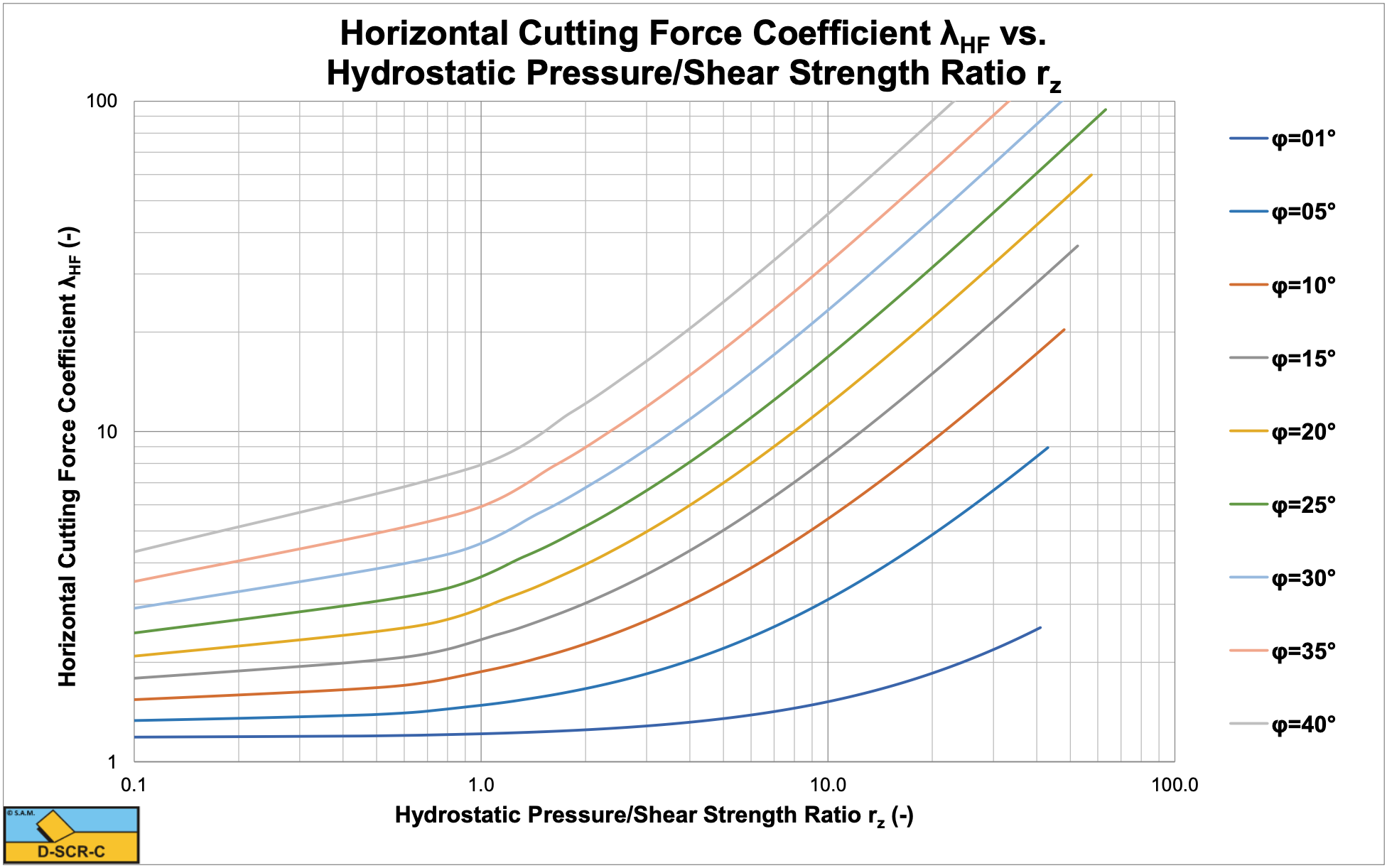
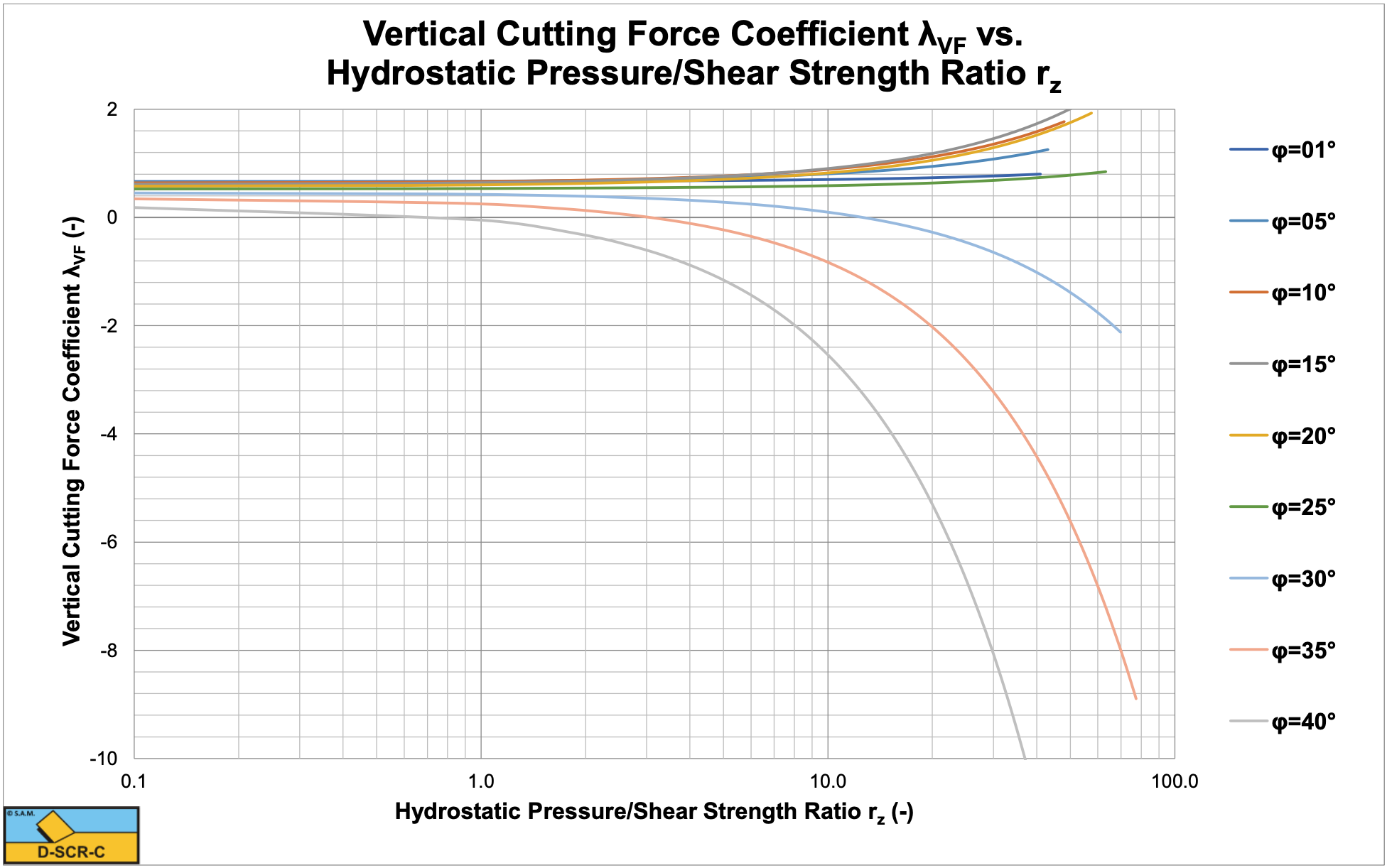
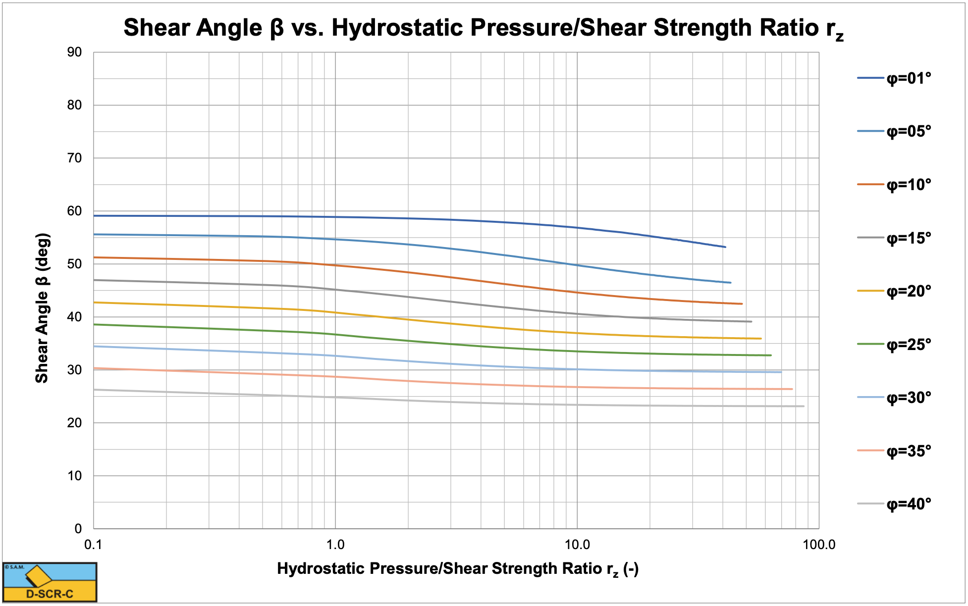
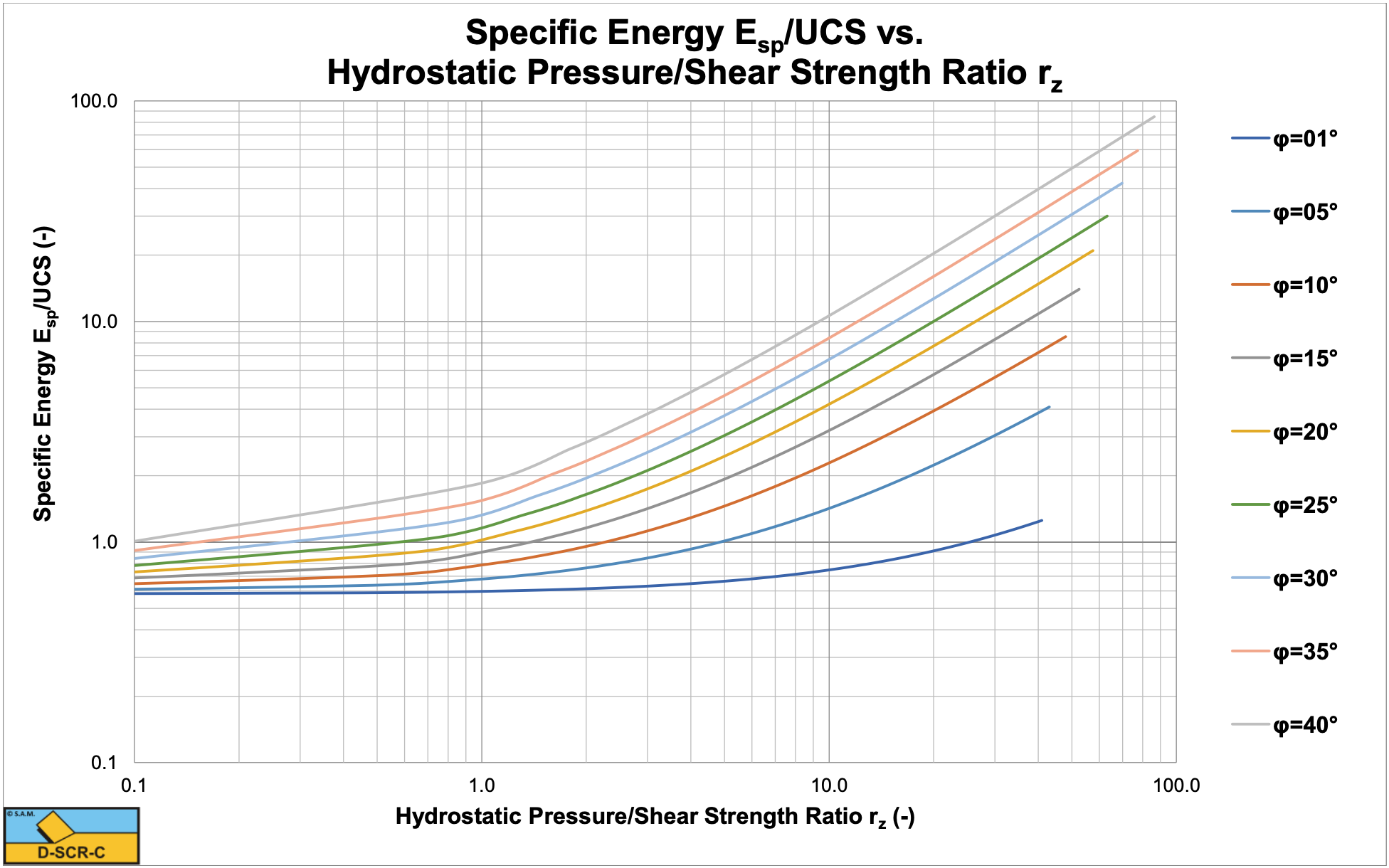
Figure 9-9, Figure 9-10 and Figure 9-11 show the horizontal and vertical cutting force coefficients and the shear angle as a function of the ratio of the hydrostatic pressure to the shear strength of the rock r_z for a 60 degree blade and full cavitation. If this ratio equals 1, it means the hydrostatic pressure equals the shear strength. At small ratios the resulting values approach atmospheric cutting of rock. Also at small ratios the shear angle approaches the theoretical value for atmospheric cutting. Figure 9-12 shows the E_sp/UCS ratio, which is very convenient for production estimation.

The vertical cutting force coefficient λ_VF is positive downwards directed. From the calculations it appeared that for a 60 degree blade, the Curling Type will already occur with an h_b/h_i=1. For a 110 degree blade it requires an h_b/h_i=4-5, depending on the internal friction angle. The transition at small h_b/h_i ratios, between the Flow Type and the Curling Type, will occur at blade angles between 60 and 90 degrees. So its important to determine the cutting forces for both mechanisms in order to see which of the two should be applied. This is always the mechanism resulting in the smallest horizontal cutting force.

Figure 9-9: The horizontal cutting force coefficient λ_HF for a 60 degree blade, h_b/h_i=1.

Figure 9-10: The vertical cutting force coefficient λ_VF for a 60 degree blade, h_b/h_i=1.

Figure 9-11:The shear angle β, for a 60 degree blade, h_b/h_i=1.

Figure 9-12: The E_sp/UCS ratio, for a 60 degree blade, h_b/h_i=1.