10.2: TheForceEquilibrium
- Page ID
- 29346

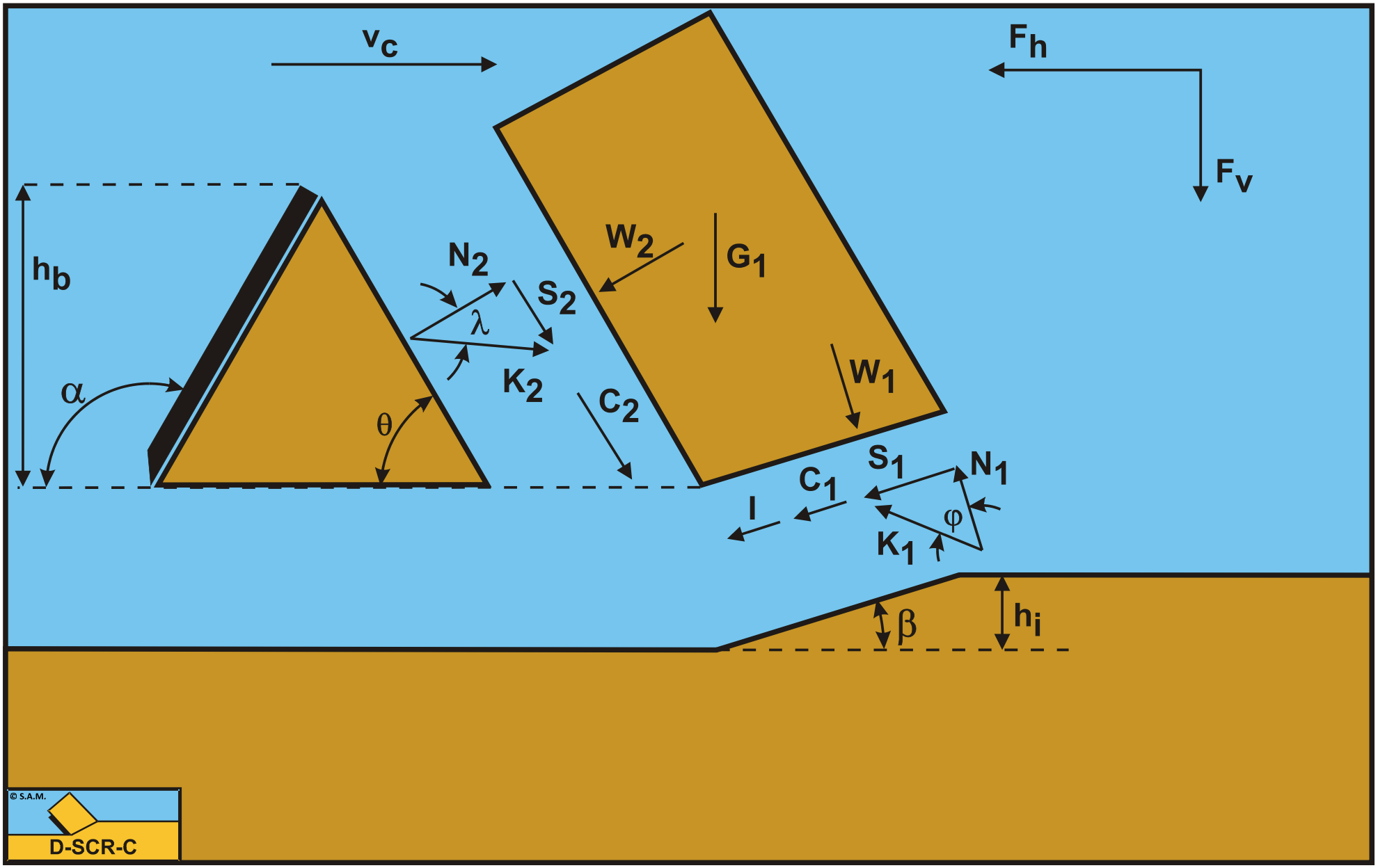
Figure 10-2 illustrates the forces on the layer of soil cut. The forces shown are valid in general for each type of soil.
The forces acting on the layer A-B are:
-
A normal force acting on the shear surface N1, resulting from the effective grain stresses.
-
A shear force S1 as a result of internal friction N1·tan(φ).
-
A force W1 as a result of water under pressure in the shear zone.
-
A shear force C1 as a result of pure cohesion \(\ \tau_\mathrm{c}\) or shear strength. This force can be calculated by multiplying the cohesive shear strength \(\ \tau_\mathrm{c}\) with the area of the shear plane.
-
A gravity force G1 as a result of the weight of the layer cut.
-
An inertial force I, resulting from acceleration of the soil.
-
A force normal to the pseudo blade N2, resulting from the effective grain stresses.
-
A shear force S2 as a result of the soil/soil friction N2·tan(λ) between the layer cut and the wedge pseudo blade. The friction angle λ does not have to be equal to the internal friction angle φ in the shear plane, since the soil has already been deformed.
-
A shear force C2 as a result of the mobilized cohesion between the soil and the wedge \(\ \tau_\mathrm{c}\). This force can be calculated by multiplying the cohesive shear strength \(\ \tau_\mathrm{c}\) of the soil with the contact area between the soil and the wedge.
- A force W2 as a result of water under pressure on the wedge.
The normal force N1 and the shear force S1 can be combined to a resulting grain force K1.
\[\ \mathrm{K}_{1}=\sqrt{\mathrm{N}_{1}^{2}+\mathrm{S}_{1}^{2}}\tag{10-1}\]
The forces acting on the wedge front or pseudo blade A-C when cutting soil, can be distinguished as:
-
A force normal to the blade N2, resulting from the effective grain stresses.
-
A shear force S2 as a result of the soil/soil friction N2·tan(λ) between the layer cut and the wedge pseudo blade. The friction angle λ does not have to be equal to the internal friction angle φ in the shear plane, since the soil has already been deformed.
-
A shear force C2 as a result of the cohesion between the layer cut and the pseudo blade \(\ \tau_\mathrm{c}\). This force can be calculated by multiplying the cohesive shear strength \(\ \tau_\mathrm{c}\) of the soil with the contact area between the soil and the pseudo blade.
-
A force W2 as a result of water under pressure on the pseudo blade A-C.
These forces are shown in Figure 10-3. If the forces N2 and S2 are combined to a resulting force K2 and the adhesive force and the water under pressures are known, then the resulting force K2 is the unknown force on the blade. By taking the horizontal and vertical equilibrium of forces an expression for the force K2 on the blade can be derived.
\[\ \mathrm{K}_{2}=\sqrt{\mathrm{N}_{2}^{2}+\mathrm{S}_{2}^{2}}\tag{10-2}\]
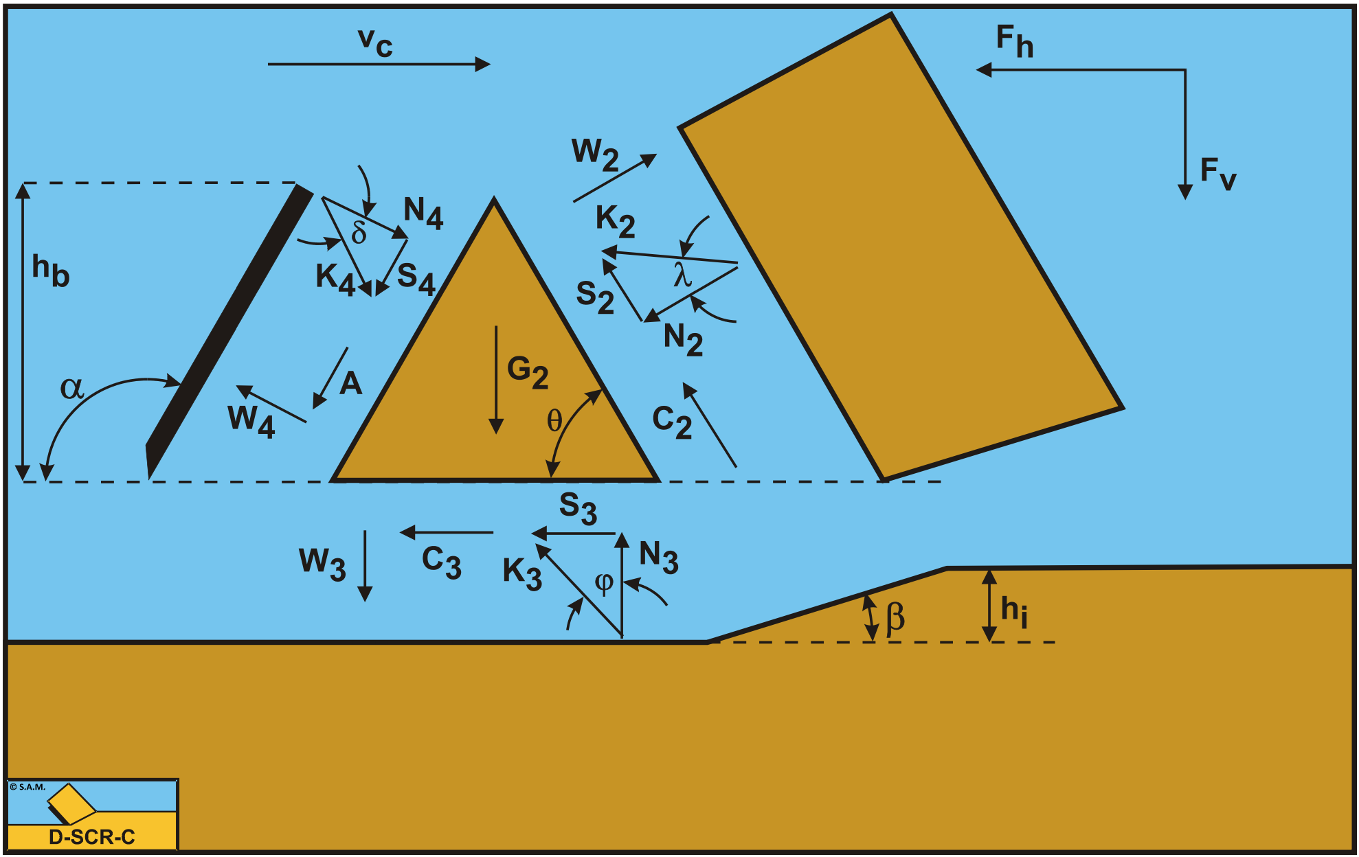
The forces acting on the wedge bottom A-D when cutting soil, can be distinguished as:
-
A force N3, resulting from the effective grain stresses, between the wedge bottom and the undisturbed soil.
-
A shear force S3 as a result of the soil/soil friction N3·tan(φ) between the wedge bottom and the undisturbed soil.
-
A shear force C3 as a result of the cohesion between the wedge bottom and the undisturbed soil \(\ \tau_\mathrm{c}\). This force can be calculated by multiplying the cohesive shear strength \(\ \tau_\mathrm{c}\) of the soil with the contact area between the wedge bottom and the undisturbed soil.
-
A force W3 as a result of water under pressure on the wedge bottom A-D.
The normal force N3 and the shear force S3 can be combined to a resulting grain force K3.
\[\ \mathrm{K}_{3}=\sqrt{\mathrm{N}_{3}^{2}+\mathrm{S}_{3}^{2}}\tag{10-3}\]
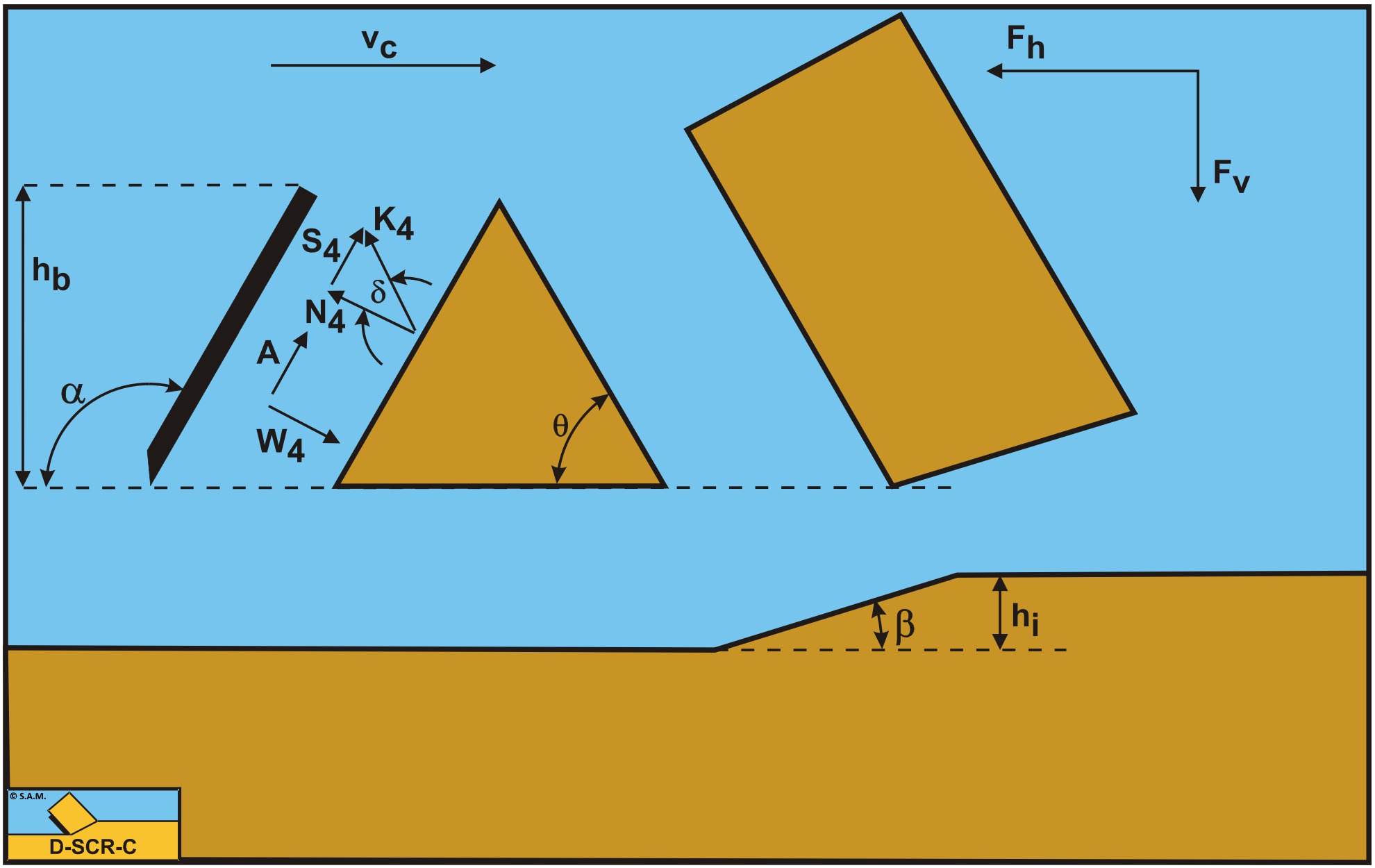
The forces acting on a straight blade C-D when cutting soil (see Figure 10-4), can be distinguished as:
-
A force normal to the blade N4, resulting from the effective grain stresses.
-
A shear force S4 as a result of the soil/steel friction N4·tan(δ).
-
A shear force A as a result of pure adhesion between the soil and the blade \(\ \tau_\mathrm{a}\). This force can be calculated by multiplying the adhesive shear strength \(\ \tau_\mathrm{a}\) of the soil with the contact area between the soil and the blade.
The normal force N4 and the shear force S4 can be combined to a resulting grain force K4.
\[\ \mathrm{K}_{4}=\sqrt{\mathrm{N}_{4}^{2}+\mathrm{S}_{4}^{2}}\tag{10-4}\]
The horizontal equilibrium of forces on the layer cut:
\[\ \sum \mathrm{F}_{\mathrm{h}}=\mathrm{K}_{1} \cdot \sin (\beta+\varphi)-\mathrm{W}_{1} \cdot \sin (\beta)+\mathrm{C}_{1} \cdot \cos (\beta)+\mathrm{I} \cdot \cos (\beta)
-\mathrm{C}_{2} \cdot \cos (\theta)+\mathrm{W}_{2} \cdot \sin (\theta)-\mathrm{K}_{2} \cdot \sin (\theta+\lambda)=\mathrm{0}\tag{10-5}\]
The vertical equilibrium of forces on the layer cut:
\[\ \sum \mathrm{F}_{\mathrm{v}}=-\mathrm{K}_{1} \cdot \cos (\beta+\varphi)+\mathrm{W}_{1} \cdot \cos (\beta)+\mathrm{C}_{1} \cdot \sin (\beta)+\mathrm{I} \cdot \sin (\beta)+\mathrm{G}_{1}+\mathrm{C}_{2} \cdot \sin (\theta)+\mathrm{W}_{2} \cdot \cos (\theta)-\mathrm{K}_{2} \cdot \cos (\theta+\lambda)=\mathrm{0} \tag{10-6}\]
The force K1 on the shear plane is now:
\[\ \mathrm{K}_{1}= \frac{\mathrm{W}_{2} \cdot \sin (\lambda)+\mathrm{W}_{1} \cdot \sin (\theta+\beta+\lambda)+\mathrm{G}_{1} \cdot \sin (\theta+\lambda)-\mathrm{I} \cdot \cos (\theta+\beta+\lambda)}{\sin (\theta+\beta+\lambda+\varphi)} +\frac{-\mathrm{C}_{1} \cdot \cos (\theta+\beta+\lambda)+\mathrm{C}_{2} \cdot \cos (\lambda)}{\sin (\theta+\beta+\lambda+\varphi)}\tag{10-7} \]
The force K2 on the pseudo blade is now:
\[\ \mathrm{K}_{2}= \frac{\mathrm{W}_{2} \cdot \sin (\theta+\beta+\varphi)+\mathrm{W}_{1} \cdot \sin (\varphi)+\mathrm{G}_{1} \cdot \sin (\beta+\varphi)+\mathrm{I} \cdot \cos (\varphi)}{\sin (\theta+\beta+\lambda+\varphi)} +\frac{+\mathrm{C}_{1} \cdot \cos (\varphi)-\mathrm{C}_{2} \cdot \cos (\theta+\beta+\varphi)}{\sin (\theta+\beta+\lambda+\varphi)} \tag{10-8}\]
From equation (10-8) the forces on the pseudo blade can be derived. On the pseudo blade a force component in the direction of cutting velocity Fh and a force perpendicular to this direction Fv can be distinguished.
\[\ \mathrm{F_{h}=-W_{2} \cdot \sin (\theta)+K_{2} \cdot \sin (\theta+\lambda)+C_{2} \cdot \cos (\theta)}\tag{10-9}\]
\[\ \mathrm{F}_{v}=-\mathrm{W}_{2} \cdot \cos (\theta)+\mathrm{K}_{2} \cdot \cos (\theta+\lambda)-\mathrm{C}_{2} \cdot \sin (\theta)\tag{10-10}\]
The normal force on the shear plane is now:
\[\ \mathrm{N}_{1}= \frac{\mathrm{W}_{2} \cdot \sin (\lambda)+\mathrm{W}_{1} \cdot \sin (\theta+\beta+\lambda)+\mathrm{G}_{1} \cdot \sin (\theta+\lambda)}{\sin (\theta+\beta+\lambda+\varphi)} \cdot \cos (\varphi) +\frac{-\mathrm{I} \cdot \cos (\theta+\beta+\lambda)-\mathrm{C}_{1} \cdot \cos (\theta+\beta+\lambda)+\mathrm{C}_{2} \cdot \cos (\lambda)}{\sin (\theta+\beta+\lambda+\varphi)} \cdot \cos (\varphi)\tag{10-11}\]
The normal force on the pseudo blade is now:
\[\ \mathrm{N}_{2}= \frac{\mathrm{W}_{2} \cdot \sin (\theta+\beta+\varphi)+\mathrm{W}_{1} \cdot \sin (\varphi)+\mathrm{G}_{1} \cdot \sin (\beta+\varphi)}{\sin (\theta+\beta+\lambda+\varphi)} \cdot \cos (\lambda) +\frac{+\mathrm{I} \cdot \cos (\varphi)+\mathrm{C}_{1} \cdot \cos (\varphi)-\mathrm{C}_{2} \cdot \cos (\theta+\beta+\varphi)}{\sin (\theta+\beta+\lambda+\varphi)} \cdot \cos (\lambda)\tag{10-12} \]
Now knowing the forces on the pseudo blade A-C, the equilibrium of forces on the wedge A-C-D can be derived. The horizontal equilibrium of forces on the wedge is:
\[\ \sum \mathrm{F}_{\mathrm{h}}=-\mathrm{A} \cdot \cos (\alpha)+\mathrm{W}_{4} \cdot \sin (\alpha)-\mathrm{K}_{4} \cdot \sin (\alpha+\delta)+\mathrm{K}_{3} \cdot \sin (\varphi) +\mathrm{C}_{3}-\mathrm{W}_{2} \cdot \sin (\theta)+\mathrm{C}_{2} \cdot \cos (\theta)+\mathrm{K}_{2} \cdot \sin (\theta+\lambda)=\mathrm{0} \tag{10-13}\]
The vertical equilibrium of forces on the wedge is:
\[\ \sum \mathrm{F}_{\mathrm{v}}=\mathrm{A} \cdot \sin (\alpha)+\mathrm{W}_{4} \cdot \cos (\alpha)-\mathrm{K}_{4} \cdot \cos (\alpha+\delta)+\mathrm{W}_{3}-\mathrm{K}_{3} \cdot \cos (\varphi)
-\mathrm{W}_{2} \cdot \cos (\theta)-\mathrm{C}_{2} \cdot \sin (\theta)+\mathrm{K}_{2} \cdot \cos (\theta+\lambda)+\mathrm{G}_{2}=\mathrm{0}\tag{10-14}\]
The unknowns in this equation are K3 and K4, since K2 has already been solved. Three other unknowns are the adhesive force on the blade A, since the adhesion does not have to be mobilized fully if the wedge is static, the external friction angle δ, since also the external friction does not have to be fully mobilized, and the wedge angle θ. These 3 additional unknowns require 3 additional conditions in order to solve the problem. One additional condition is the equilibrium of moments of the wedge, a second condition the principle of minimum required cutting energy. A third condition is found by assuming that the external shear stress (adhesion) and the external shear angle (external friction) are mobilized by the same amount. Depending on whether the soil pushes upwards or downwards against the blade, the mobilization factor is between -1 and +1. Now in practice, sand and rock have no adhesion while clay has no external friction, so in these cases the third condition is not relevant. However in mixed soil both the external shear stress and the external friction may be present.
The force K3 on the bottom of the wedge is now:
\[\ \begin{array}{left} \mathrm{K}_{3}&= \frac{-\mathrm{W}_{2} \cdot \sin (\alpha+\delta-\theta)+\mathrm{W}_{3} \cdot \sin (\alpha+\delta)+\mathrm{W}_{4} \cdot \sin (\delta)}{\sin (\alpha+\delta+\varphi)} \\&+\frac{\mathrm{K}_{2} \cdot \sin (\alpha+\delta-\theta-\lambda)+\mathrm{G}_{2} \cdot \sin (\alpha+\delta)}{\sin (\alpha+\delta+\varphi)} \\&+\frac{\mathrm{A} \cdot \cos (\delta)+\mathrm{C}_{3} \cdot \cos (\alpha+\delta)-\mathrm{C}_{2} \cdot \cos (\alpha+\delta-\theta)}{\sin (\alpha+\delta+\varphi)} & \end{array}\tag{10-15}\]
The force K4 on the blade is now:
\[\ \begin{array}{left} \mathrm{K}_{4}=& \frac{-\mathrm{W}_{2} \cdot \sin (\theta+\varphi)+\mathrm{W}_{3} \cdot \sin (\varphi)+\mathrm{W}_{4} \cdot \sin (\alpha+\varphi)+\mathrm{K}_{2} \cdot \sin (\theta+\lambda+\varphi)+\mathrm{G}_{2} \cdot \sin (\varphi)}{\sin (\alpha+\delta+\varphi)} \\ &+\frac{-\mathrm{A} \cdot \cos (\alpha+\varphi)+\mathrm{C}_{3} \cdot \cos (\varphi)+\mathrm{C}_{2} \cdot \cos (\theta+\varphi)}{\sin (\alpha+\delta+\varphi)} \end{array}\tag{10-16}\]
This results in a horizontal force of:
\[\ \mathrm{F}_{\mathrm{h}}=-\mathrm{W}_{\mathrm{4}} \cdot \sin (\alpha)+\mathrm{K}_{4} \cdot \sin (\alpha+\delta)+\mathrm{A} \cdot \cos (\alpha)\tag{10-17}\]
And in a vertical force of:
\[\ \mathrm{F}_{\mathrm{v}}=-\mathrm{W}_{\mathrm{4}} \cdot \cos (\alpha)+\mathrm{K}_{4} \cdot \cos (\alpha+\delta)-\mathrm{A} \cdot \sin (\alpha)\tag{10-18}\]