12.3: Pore Pressures

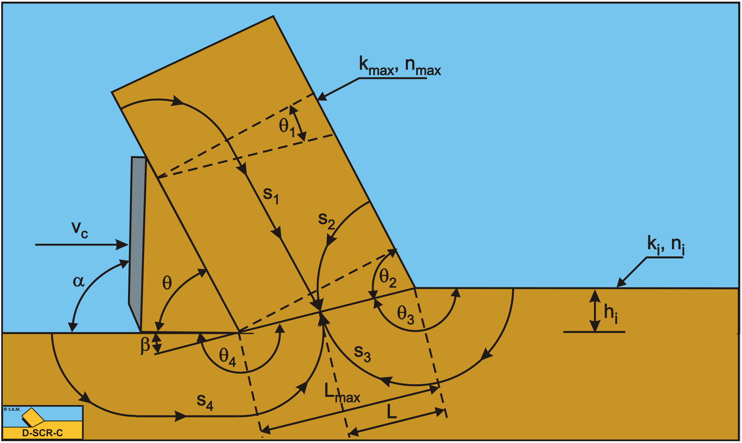
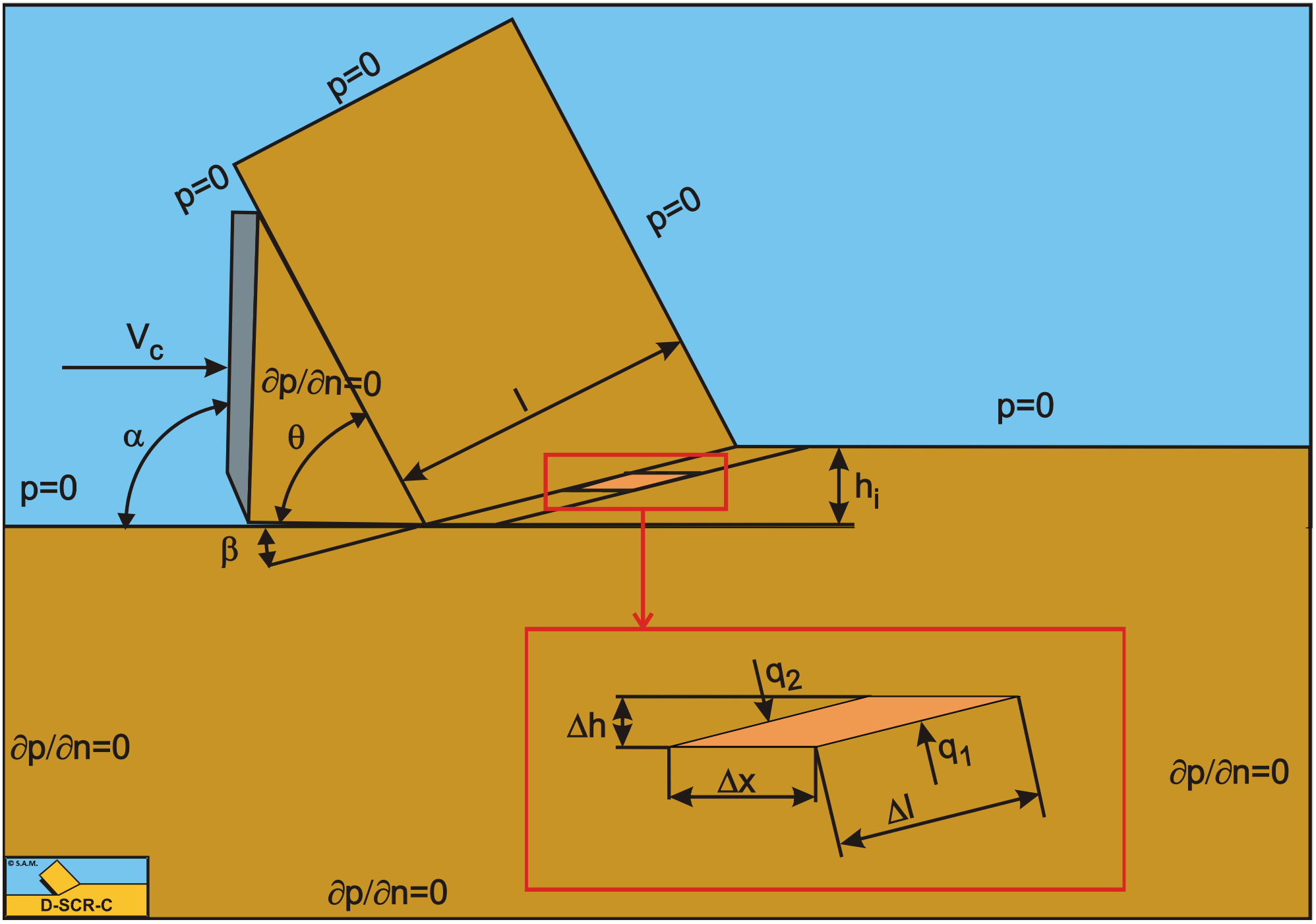
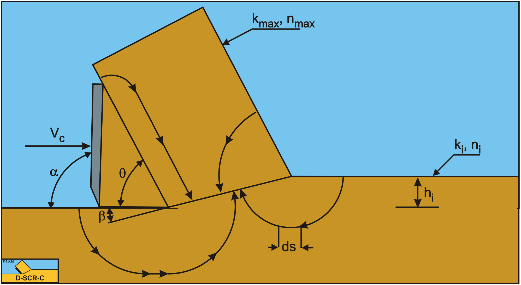
If the cutting process is assumed to be stationary, the water flow through the pores of the sand can be described in a blade motions related coordinate system. The determination of the water vacuum pressures in the sand around the blade is then limited to a mixed boundary conditions problem. The potential theory can be used to solve this problem. For the determination of the water vacuum pressures it is necessary to have a proper formulation of the boundary condition in the shear zone. Miedema (1985A) derived the basic equation for this boundary condition. In later publications a more extensive derivation is published. If it is assumed that no deformations take place outside the deformation zone, then:

\[\ \left|\frac{\partial^{2} \mathrm{p}}{\partial \mathrm{x}^{2}}\right|+\left|\frac{\partial^{2} \mathrm{p}}{\partial \mathrm{y}^{2}}\right|=\mathrm{0}\tag{12-15}\]

Making the boundary condition in the shear plane dimensionless is similar to that of the breach equation of Meijer and Van Os (1976). In the breach problem the length dimensions are normalized by dividing them by the breach height, while in the cutting of sand they are normalized by dividing them by the cut layer thickness. Equation (12-15) is the same as the equation without a wedge. In the shear plane A-B the following equation is valid:

\[\ \frac{\mathrm{k}_{\mathrm{i}}}{\mathrm{k}_{\mathrm{m a x}}} \cdot\left|\frac{\partial \mathrm{p}}{\partial \mathrm{n}^{\prime}}\right|_{\mathrm{1}}+\left|\frac{\partial \mathrm{p}}{\partial \mathrm{n}^{\prime}}\right|_{\mathrm{2}}=\frac{\rho_{\mathrm{w}} \cdot \mathrm{g} \cdot \mathrm{v}_{\mathrm{c}} \cdot \varepsilon \cdot \mathrm{h}_{\mathrm{i}} \cdot \sin (\beta)}{\mathrm{k}_{\mathrm{m a x}}} \quad\text{ with: }\quad \mathrm{n}^{\prime}=\frac{\mathrm{n}}{\mathrm{h}_{\mathrm{i}}}\tag{12-16}\]

This equation is made dimensionless with:

\[\ \left|\frac{\partial \mathrm{p}}{\partial \mathrm{n}}\right|^{\prime}=\frac{\left|\frac{\partial \mathrm{p}}{\partial \mathrm{n}^{\prime}}\right|}{\rho_{\mathrm{w}} \cdot \mathrm{g} \cdot \mathrm{v}_{\mathrm{c}} \cdot \varepsilon \cdot \mathrm{h}_{\mathrm{i}} / \mathrm{k}_{\mathrm{m a x}}}\tag{12-17}\]

The accent indicates that a certain variable or partial derivative is dimensionless. The next dimensionless equation is now valid as a boundary condition in the deformation zone:

\[\ \frac{\mathrm{k}_{\mathrm{i}}}{\mathrm{k}_{\mathrm{m a x}}} \cdot\left|\frac{\partial \mathrm{p}}{\partial \mathrm{n}}\right|_{\mathrm{1}}+\left|\frac{\partial \mathrm{p}}{\partial \mathrm{n}}\right|_{\mathrm{2}}=\sin (\beta)\tag{12-18}\]

The storage equation also has to be made dimensionless, which results in the next equation:

\[\ \left|\frac{\partial^{2} \mathrm{p}}{\partial \mathrm{x}^{2}}\right|+\left|\frac{\partial^{2} \mathrm{p}}{\partial \mathrm{y}^{2}}\right|^{\prime}=\mathrm{0}\tag{12-19}\]

Because this equation equals zero, it is similar to equation (12-15). The water under-pressures distribution in the sand package can now be determined using the storage equation and the boundary conditions. Because the calculation of the water under-pressures is dimensionless the next transformation has to be performed to determine the real water under-pressures. The real water under-pressures can be determined by integrating the derivative of the water under-pressures in the direction of a flow line, along a flow line, so:

\[\ \mathrm{P}_{\mathrm{c a l c}}=\int_{\mathrm{s^{\prime}}}\left|\frac{\partial \mathrm{p}}{\partial \mathrm{s}}\right|^{\prime} \cdot \mathrm{d s}^{\prime}\tag{12-20}\]

This is illustrated in Figure 12-7 and Figure 12-8. Using equation (12-20) this is written as:

\[\ \mathrm{P}_{\text {real }}=\int_{\mathrm{s}}\left|\frac{\partial \mathrm{p}}{\partial \mathrm{s}}\right| \cdot \mathrm{d s}=\int_{\mathrm{s}^{\prime}} \frac{\rho_{\mathrm{w}} \cdot \mathrm{g} \cdot \mathrm{v}_{\mathrm{c}} \cdot \varepsilon \cdot \mathrm{h}_{\mathrm{i}}}{\mathrm{k}_{\mathrm{m a x}}} \cdot\left|\frac{\partial \mathrm{p}}{\partial \mathrm{s}}\right|^{\prime} \cdot \mathrm{d s}^{\prime} \quad\text{ with: }\quad \mathrm{s}^{\prime}=\frac{\mathrm{s}}{\mathrm{h}_{\mathrm{i}}}\tag{12-21}\]

This gives the next relation between the real emerging water under pressures and the calculated water under pressures:

\[\ \mathrm{P}_{\text {real }}=\frac{\rho_{\mathrm{w}} \cdot \mathrm{g} \cdot \mathrm{v}_{\mathrm{c}} \cdot \varepsilon \cdot \mathrm{h}_{\mathrm{i}}}{\mathrm{k}_{\mathrm{m a x}}} \cdot \mathrm{P}_{\mathrm{c a l c}}\tag{12-22}\]

Figure 12-7: The volume balance over the shear zone.

Figure 12-8: Possible flow lines.

To be independent of the ratio between the initial permeability k_i and the maximum permeability k_max , k_max has to be replaced with the weighted average permeability k_m before making the measured water under pressures dimensionless.

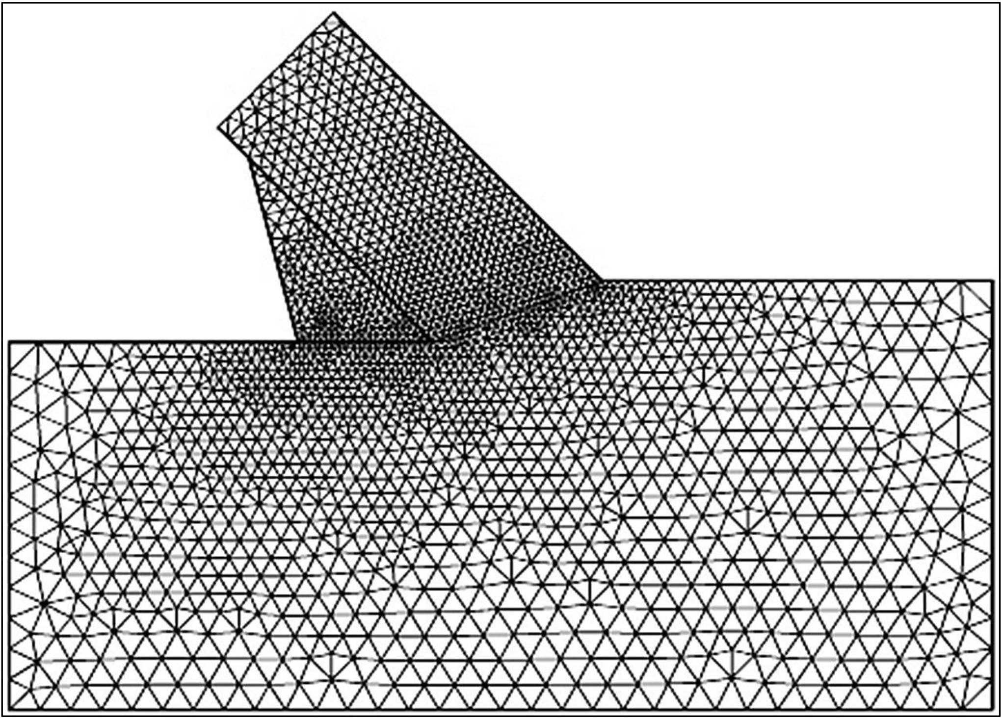
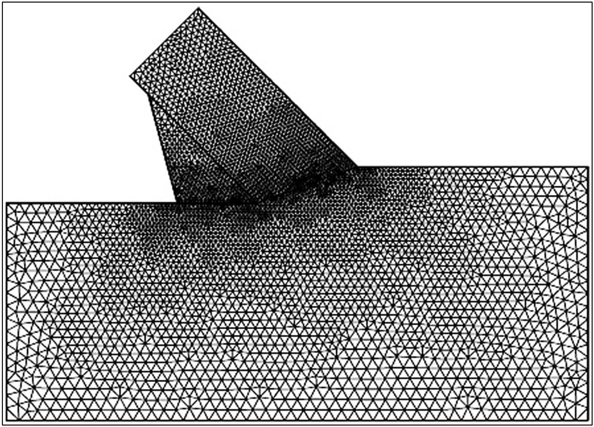
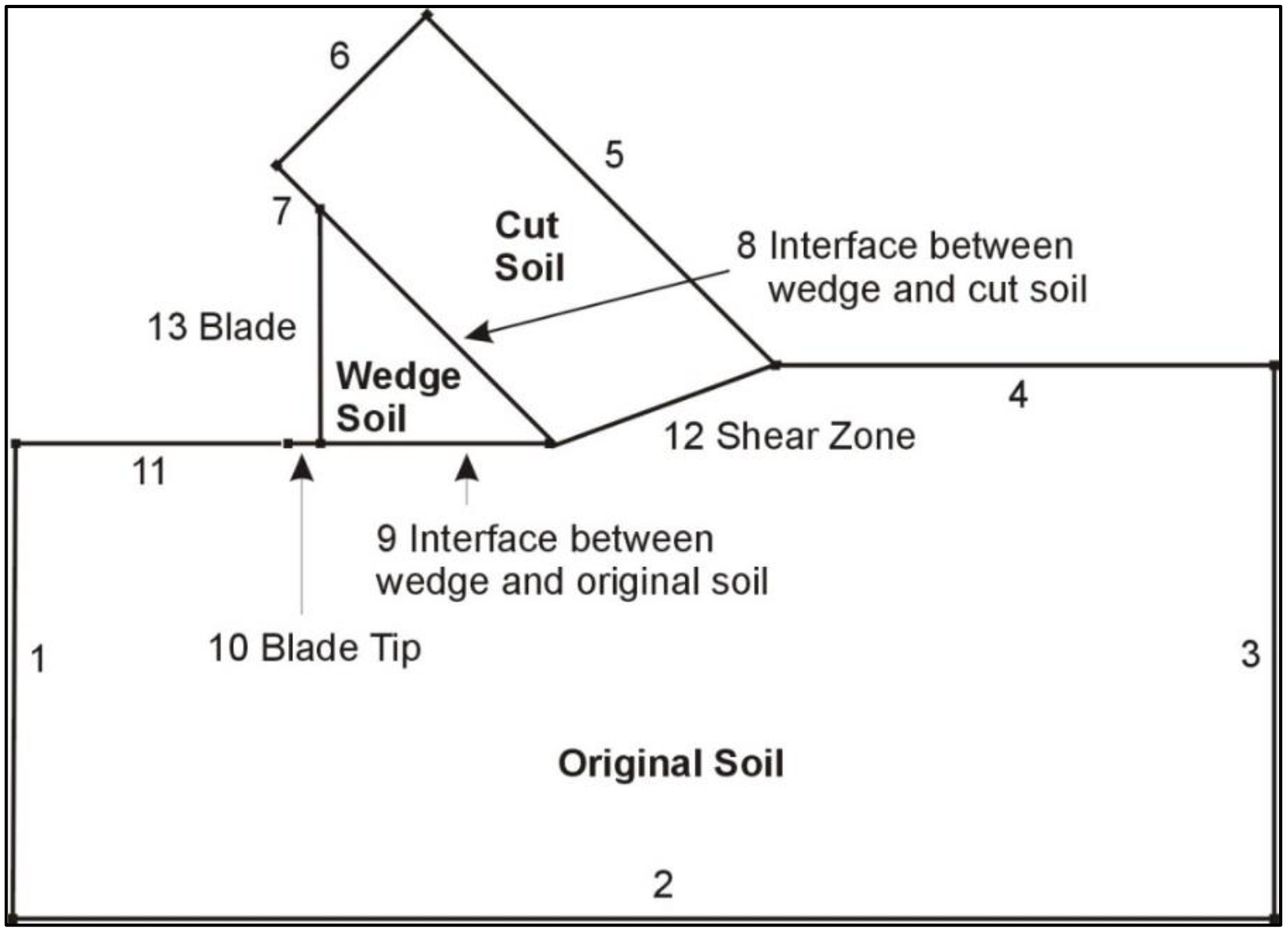
The water vacuum pressures in the sand package on and around the blade are numerically determined using the finite element method. A standard FEM software package is used (Segal (2001)). Within this package and the use of the available "subroutines" a program is written, with which water vacuum pressures can be calculated and be output graphically and numerically. As shown in Figure 12-9, the SEPRAN model is made up of three parts, the original sand layer, the cut sand layer, and the wedge. The solution of such a calculation is however not only dependent on the physical model of the problem, but also on the next points:

1. The size of the area in which the calculation takes place.

2. The size and distribution of the elements

3. The boundary conditions

The choices for these three points have to be evaluated with the problem that has to be solved in mind. These calculations are about the values and distribution of the water under-pressures in the shear zone and on the blade, on the interface between wedge and cut sand, between wedge and the original sand layer. A variation of the values for point 1 and 2 may therefore not influence this part of the solution. This is achieved by on one hand increasing the area in which the calculations take place in steps and on the other hand by decreasing the element size until the variation in the solution was less than 1%. The distribution of the elements is chosen such that a finer mesh is present around the blade tip, the shear zone and on the blade, also because of the blade tip problem. A number of boundary conditions follow from the physical model of the cutting process, these are:

• For the hydrostatic pressure it is valid to take a zero pressure as the boundary condition.

• The boundary conditions along the boundaries of the area where the calculation takes place that are located in the sand package are not determined by the physical process.

• For this boundary condition there is a choice among:

1. A hydrostatic pressure along the boundary.

2. A boundary as an impermeable wall.

3. A combination of a known pressure and a known specific flow rate.

Figure 12-9: The boundaries of the FEM model.

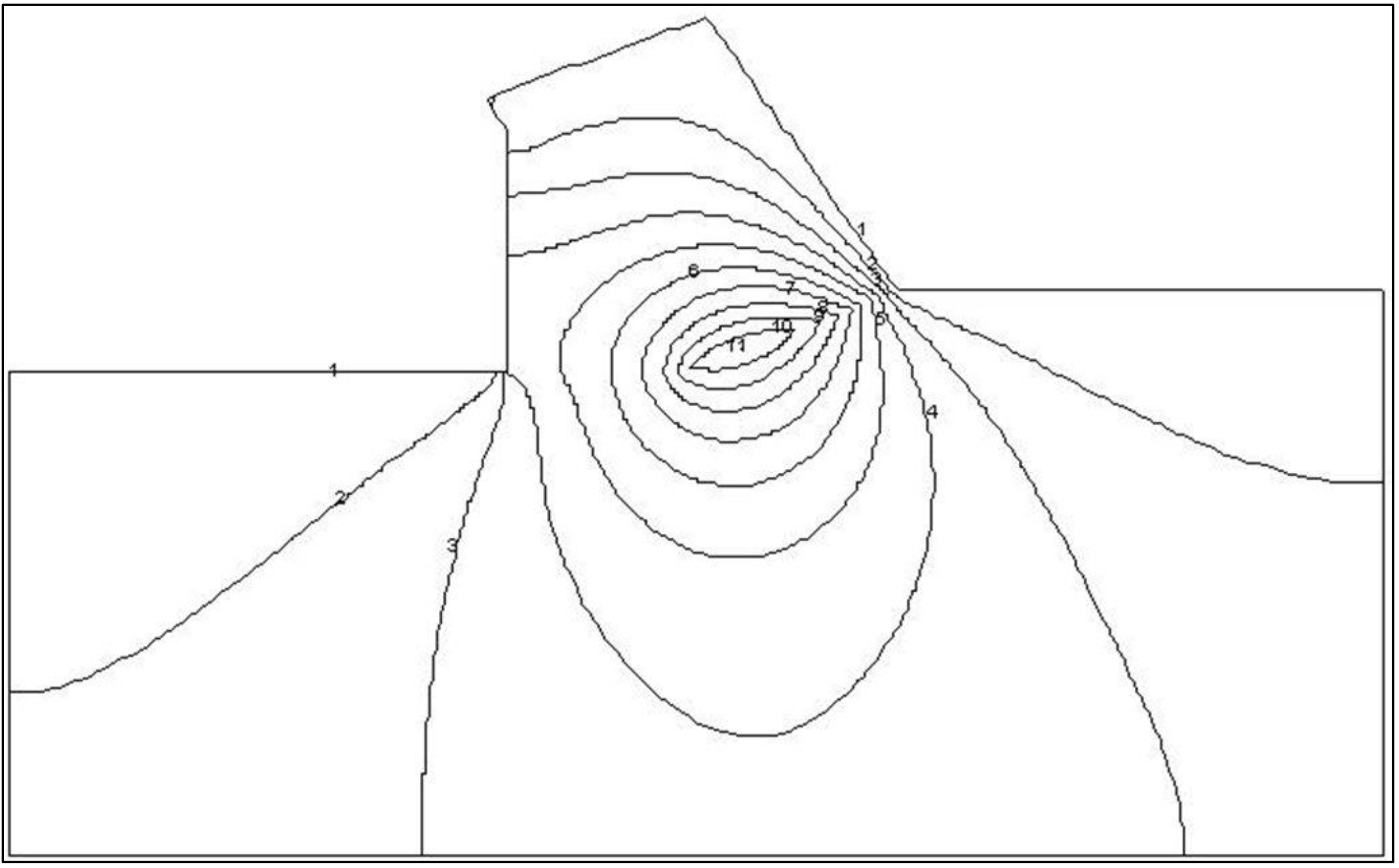
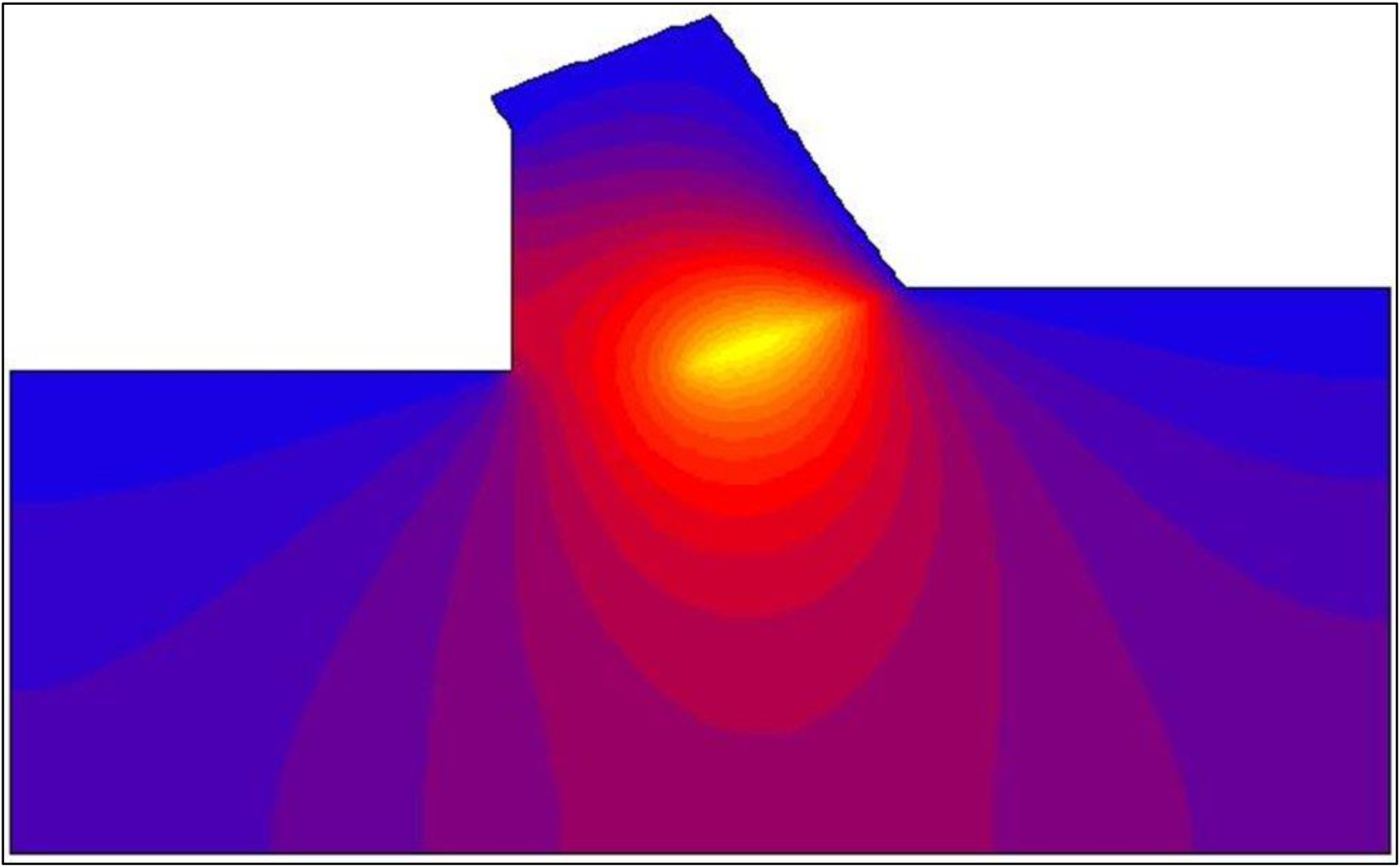
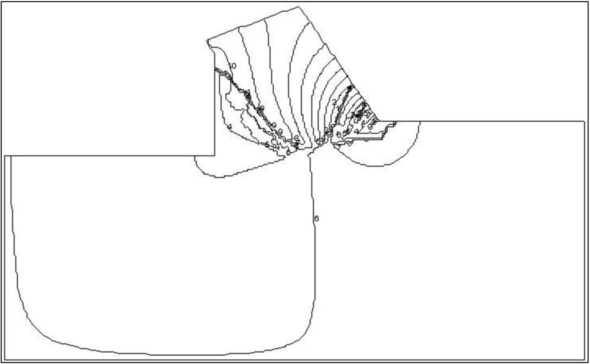
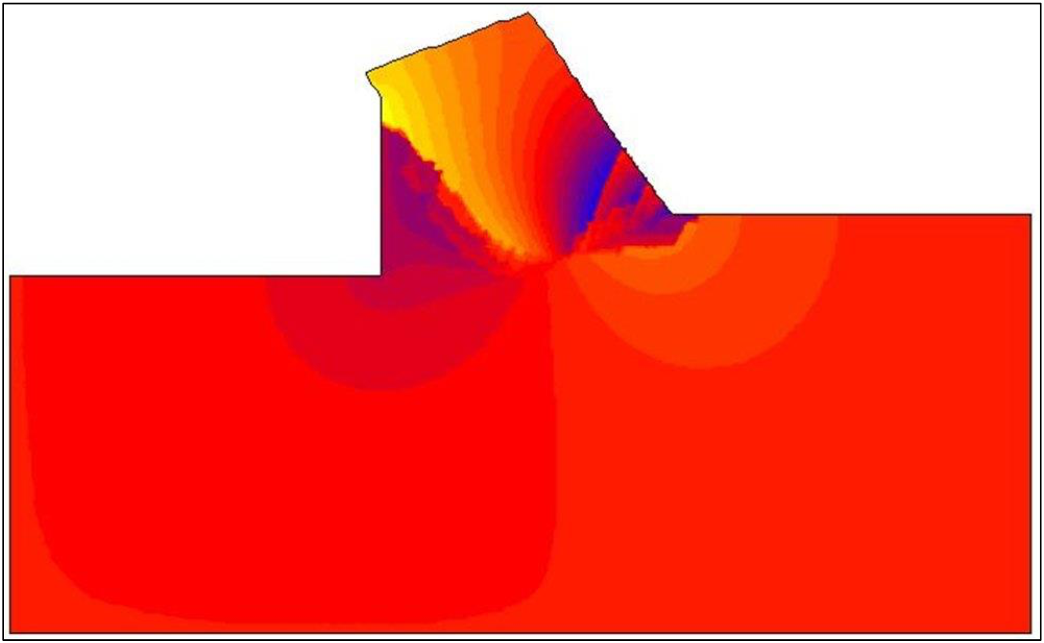
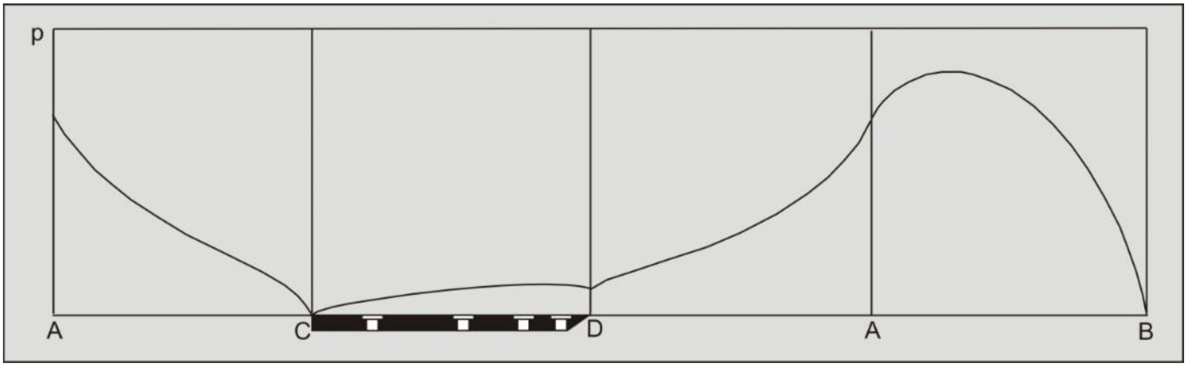
None of these choices complies with the real process. Water from outside the calculation area will flow through the boundary. This also implies, however, that the pressure along this boundary is not hydrostatic. If, however, the boundary is chosen with enough distance from the real cutting process the boundary condition may not have an influence on the solution. The impermeable wall is chosen although this choice is arbitrary. Figure 12-14 and Figure 12-16 give an impression of the equipotential lines and the stream lines in the model area. Figure 12-10 show the dimensionless pore pressure distributions on the lines A-B, A-C, A-D and D-C. The average dimensionless pore pressures on these lines are named p_1m, p_2m, p_3m and p_4m.

Figure 12-10: Pore pressure distribution on the shear plane A-B, the bottom of the wedge A-D, the blade D-C and the front of the wedge A-C.

If there is no cavitation the water pressures forces W₁, W₂, W₃ and W₄ can be written as:

\[\ \mathrm{W}_{1}=\frac{\mathrm{p}_{1 \mathrm{m}} \cdot \rho_{\mathrm{w}} \cdot \mathrm{g} \cdot \mathrm{v}_{\mathrm{c}} \cdot \varepsilon \cdot \mathrm{h}_{\mathrm{i}}^{2} \cdot \mathrm{w}}{\mathrm{k}_{\max } \cdot \sin (\beta)}\tag{12-23}\]

And

\[\ \mathrm{W}_{2}=\frac{\mathrm{p}_{2 \mathrm{m}} \cdot \rho_{\mathrm{w}} \cdot \mathrm{g} \cdot \mathrm{v}_{\mathrm{c}} \cdot \mathrm{\varepsilon} \cdot \mathrm{h}_{\mathrm{i}} \cdot \mathrm{h}_{\mathrm{b}} \cdot \mathrm{w}}{\mathrm{k}_{\mathrm{m a x}} \cdot \sin (\theta)}\tag{12-24}\]

And

\[\ \mathrm{W}_{3}=\frac{\mathrm{p}_{3 \mathrm{m}} \cdot \rho_{\mathrm{w}} \cdot \mathrm{g} \cdot \mathrm{v}_{\mathrm{c}} \cdot \varepsilon \cdot \mathrm{h}_{\mathrm{i}} \cdot \mathrm{h}_{\mathrm{b}} \cdot \mathrm{w}}{\mathrm{k}_{\mathrm{m a x}}} \cdot\left(\frac{\cos (\theta)}{\sin (\theta)}-\frac{\cos (\alpha)}{\sin (\alpha)}\right)\tag{12-25}\]

And

\[\ \mathrm{W}_{4}=\frac{\mathrm{p}_{4 \mathrm{m}} \cdot \rho_{\mathrm{w}} \cdot \mathrm{g} \cdot \mathrm{v}_{\mathrm{c}} \cdot \varepsilon \cdot \mathrm{h}_{\mathrm{i}} \cdot \mathrm{h}_{\mathrm{b}} \cdot \mathrm{w}}{\mathrm{k}_{\max } \cdot \sin (\mathrm{\alpha})}\tag{12-26}\]

In case of cavitation W₁, W₂, W₃ and W₄ become:

\[\ \mathrm{W}_{1}=\frac{\rho_{\mathrm{w}} \cdot \mathrm{g} \cdot(\mathrm{z}+\mathrm{1 0}) \cdot \mathrm{h}_{\mathrm{i}} \cdot \mathrm{w}}{\sin (\beta)}\tag{12-27}\]

And

\[\ \mathrm{W}_{2}=\frac{\rho_{\mathrm{w}} \cdot \mathrm{g} \cdot(\mathrm{z}+\mathrm{1 0}) \cdot \mathrm{h}_{\mathrm{b}} \cdot \mathrm{w}}{\sin (\theta)}\tag{12-28}\]

And

\[\ \mathrm{W}_{3}=\frac{\rho_{\mathrm{w}} \cdot \mathrm{g} \cdot(\mathrm{z}+\mathrm{1 0}) \cdot \mathrm{h}_{\mathrm{b}} \cdot \mathrm{w}}{\mathrm{1}} \cdot\left(\frac{\cos (\theta)}{\sin (\theta)}-\frac{\cos (\alpha)}{\sin (\alpha)}\right)\tag{12-29}\]

And

\[\ \mathrm{W}_{4}=\frac{\rho_{\mathrm{w}} \cdot \mathrm{g} \cdot(\mathrm{z}+\mathrm{1 0}) \cdot \mathrm{h}_{\mathrm{b}} \cdot \mathrm{w}}{\sin (\alpha)}\tag{12-30}\]

Figure 12-11: The parallel resistor method.

Figure 12-12: The coarse mesh.

Figure 12-13: The fine mesh.

Figure 12-14: Equipotential lines of pore pressures.

Figure 12-15: Equipotential distribution in color.

Figure 12-16: The flow lines or stream function.

Figure 12-17: The stream function in colors.