3.3: Cartesian Tensors
- Page ID
- 18059
We have seen how to represent a vector in a rotated coordinate system. Can we do the same for a matrix? The basic idea is to identify a mathematical operation that the matrix represents, then require that it represent the same operation in the new coordinate system. We’ll do this in two ways: first, by seeing the matrix as a geometrical transformation of a vector, and second by seeing it as a recipe for a bilinear product of two vectors.
3.3.1 Derivation #1: preserving geometrical transformations
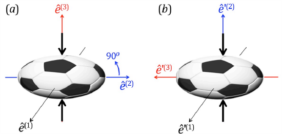
In section 3.1.1, we saw how a matrix can be regarded as a geometric transformation that acts on any vector or set of vectors (such as those that terminate on the unit circle). Look carefully at figure \(\PageIndex{1}a\). Originally spherical, the ball is compressed in the \(\hat{e}^{(3)}\) direction to half its original radius, and is therefore expanded in the \(\hat{e}^{(1)}\) and \(\hat{e}^{(2)}\) directions by a factor \(\sqrt{2}\) (so that the volume is unchanged). The strain, or change of shape, can be expressed by the matrix transformation \(\underset{\sim}{A}\):
\[\underset{\sim}{A}=\left[\begin{array}{ccc}
\sqrt{2} & 0 & 0 \\
0 & \sqrt{2} & 0 \\
0 & 0 & 1 / 2
\end{array}\right] \nonumber \]
Note that \(\det(\underset{\sim}{A})=1\).
Now suppose we rotate our coordinate system by 90° about \(\hat{e}^{(1)}\), so that \(\hat{e}^{\prime(3)}= −\hat{e}^{(2)}\) and \(\hat{e}^{\prime(2)}=\hat{e}^{(3)}\) (figure \(\PageIndex{1}b\)). In the new coordinate system, the compression is aligned in the \(\hat{e}^{\prime(2)}\) direction. We therefore expect that the matrix will look like this:
\[\underset{\sim}{A^{\prime}}=\left[\begin{array}{ccc}
\sqrt{2} & 0 & 0 \\
0 & 1 / 2 & 0 \\
0 & 0 & \sqrt{2}
\end{array}\right]\label{eq:1} \]
The compression represented by \(\underset{\sim}{A^\prime}\) is exactly the same process as that represented by \(\underset{\sim}{A}\), but but the numerical values of the matrix elements are different because the process is measured using a different coordinate system.
Can we generalize this result? In other words, given an arbitrary geometrical transformation \(\underset{\sim}{A}\), can we find the matrix \(\underset{\sim}{A^\prime}\) that represents the same transformation in an arbitrarily rotated coordinate system? Suppose that \(\underset{\sim}{A}\) transforms a general vector \(\vec{u}\) into some corresponding vector \(\vec{v}\):
\[A_{i j} u_{j}=v_{i}\label{eq:2} \]
Now we require that the same relationship be valid in an arbitrary rotated coordinate system:
\[A_{i j}^{\prime} u_{j}^{\prime}=v_{i}^{\prime}\label{eq:3} \]
What must \(\underset{\sim}{A^\prime}\) look like? To find out, we start with Equation \ref{eq:2} and substitute the reverse rotation formula 3.2.4 for \(\vec{u}\) and \(\vec{v}\):
\[A_{i j} \underbrace{u_{l}^{\prime} C_{j l}}_{u_{j}}=\underbrace{v_{k}^{\prime} C_{i k}}_{v_{i}}\label{eq:4} \]
Now we try to make Equation \(\ref{eq:4}\) look like Equation \(\ref{eq:3}\) by solving for \(\vec{v}^\prime\). Naively, you might think that you could simply divide both sides by the factor multiplying \(v^\prime_k\), namely \(C_{ik}\). This doesn’t work because, although the right hand side looks like a single term, it is really a sum of three terms with \(k = 1,2,3\), and \(C_{ik}\) has a different value in each. But instead of dividing by \(\underset{\sim}{C}\), we can multiply by its inverse. To do this, multiply both sides of Equation \(\ref{eq:4}\) by \(C_{im}\):
\[\begin{aligned}
A_{i j} u_{l}^{\prime} C_{j l} C_{i m} &=v_{k}^{\prime} C_{i k} C_{i m} \\
A_{i j} u_{l}^{\prime} C_{j l} C_{i m} &=v_{k}^{\prime} \underbrace{C_{k i}^{T} C_{i m}}_{\delta_{k m}} \\
A_{i j} C_{i m} C_{j l} u_{l}^{\prime} &=v_{m}^{\prime}
\end{aligned}. \nonumber \]
So we have successfully solved for the elements of \(\vec{v}^\prime\).
Now if Equation \(\ref{eq:3}\) holds, we can replace the right-hand side with \(A^\prime_{ml}u^\prime_l\):
\[A_{i j} C_{i m} C_{j l} u_{l}^{\prime}=A_{m l}^{\prime} u_{l}^{\prime} \nonumber \]
or
\[\left(A_{i j} C_{i m} C_{j l}-A_{m l}^{\prime}\right) u_{l}=0. \nonumber \]
This relation must be valid not just for a particular vector \(\vec{u}\) but for every vector \(\vec{u}\), and that can only be true if the quantity in parentheses is identically zero. (Make sure you understand that last statement; it will come up again.)
The transformation rule for the matrix \(\underset{\sim}{A}\) is therefore (after a minor relabelling of indices):
\[A_{i j}^{\prime}=A_{k l} C_{k i} C_{l j}\label{eq:5} \]
This transformation law can also be written in matrix form as
\[\underset{\sim}{A}^{\prime}=\underset{\sim}{C}^{T} \underset{\sim}{A} \underset{\sim}{C}\label{eq:6} \]
There is also a reverse transformation
\[A_{i j}=A_{k l}^{\prime} C_{i k} C_{j l}\label{eq:7} \]
As in the transformation of vectors, the dummy index on C\(\underset{\sim}{C}\) is in the first position for the forward transformation, in the second position for the reverse transformation.
Exercise: Use this law to check Equation \(\ref{eq:1}\).
A 2nd-order tensor is a matrix that transforms according to Equation \(\ref{eq:5}\).

3.3.2 Tensors in the laws of physics
In the above derivation of the matrix transformation formula \(\ref{eq:5}\), we thought of the vector \(\vec{u}\) as a position vector identifying, for example, a point on the surface of a soccer ball. Likewise, \(\vec{v}\) is the same point after undergoing the geometrical transformation \(\underset{\sim}{A}\), as described by Equation \(\ref{eq:2}\). We then derived Equation{\ref{eq:5}\) by assuming that the geometrical relationship between the vectors \(\vec{u}\) and \(\vec{v}\), as represented by \(\underset{\sim}{A}\), be the same in a rotated coordinate system, i.e. Equation \(\ref{eq:4})\.
Now suppose that the vectors \(\vec{u}\) and \(\vec{v}\) are not position vectors but are instead some other vector quantities such as velocity or force, and Equation \(\ref{eq:2}\) represents a physical relationship between those two vector quantities. If this relationship is to be valid for all observers (as discussed in section 3.1.2), then the matrix \(\underset{\sim}{A}\) must transform according to Equation \(\ref{eq:5}\).
A simple example is the rotational form of Newton’s second law of motion:
\[\vec{T}=\underset{\sim}{I} \vec{\alpha}\label{eq:8} \]
Here, \(\vec{\alpha}\) represents the angular acceleration of a spinning object (the rate at which its spinning motion accelerates). If \(\vec{\alpha}\) is multiplied by the matrix \(\underset{\sim}{I}\), called the moment of inertia, the result is \(\vec{T}\), the torque (rotational force) that must be applied to create the angular acceleration. If the process is viewed by two observers using different coordinate systems, their measurements of \(\underset{\sim}{I}\) are related by Equation \(\ref{eq:5}\), as is shown in appendix B. If this were not true, Equation \(eq:8\) would be useless as a law of physics and would have been discarded long ago.
The number of mathematical relationships that might conceivably exist between physical quantities is infinite, and a theoretical physicist must have some way to identify those relationships that might actually be true before spending time and money testing them in the lab. The requirement that physical laws be the same for all observers, as exemplified in Equation \(\ref{eq:5}\), plays this role. It was used extensively in Einstein’s derivation of the theory of relativity, and the modern form of the theory was inspired by that success. It is equally useful in the development of the laws of fluid dynamics as we will see shortly.
3.3.3 Derivation #2: preserving bilinear products
The dot product of two vectors \(\vec{u}\) and \(\vec{v}\) is an example of a bilinear product:
\[D(\vec{u}, \vec{v})=u_{1} v_{1}+u_{2} v_{2}+u_{3} v_{3}.\label{eq:9} \]
We call it “bilinear” because it is linear in each argument separately, e.g., \(D(\vec{a}+\vec{b},\vec{c})=D(\vec{a},\vec{c})+D(\vec{b},\vec{c})\).
With a little imagination we can invent many other bilinear products, such as
\[u_{1} v_{2}-u_{2} v_{3}+2 u_{3} v_{2}.\label{eq:10} \]
Such products can be written in the compact form
\[A_{i j} u_{i} v_{j}. \nonumber \]
For the dot product Equation \(\ref{eq:9}\), the matrix \(\underset{\sim}{A}\) is just \(\underset{\sim}{\delta}\). In the second example Equation \(\ref{eq:10}\), the matrix is
\[\underset{\sim}{A}=\left[\begin{array}{ccc}
0 & 1 & 0 \\
0 & 0 & -1 \\
0 & 2 & 0
\end{array}\right]. \nonumber \]
Write out \(A_{ij}u_iv_j\) and verify that the result is Equation \(\ref{eq:10}\).
So, every matrix can be thought of as the recipe for a bilinear product. Now suppose we rotate to a new coordinate system. How would the matrix \(\underset{\sim}{A}\) have to change so that the bilinear product it represents remains the same (i.e., is a scalar)? The following must be true:
\[A_{i j}^{\prime} u_{i}^{\prime} v_{j}^{\prime}=A_{k l} u_{k} v_{l} \nonumber \]
As in section 3.3.1, we substitute for \(\vec{u}\) and \(\vec{v}\) using the reverse rotation formula Equation \ref{eq:8}:
\[A_{i j}^{\prime} u_{i}^{\prime} v_{j}^{\prime}=A_{k l} u_{i}^{\prime} C_{k i} v_{j}^{\prime} C_{l j}. \nonumber \]
Collecting like terms, we can rewrite this as
\[\left(A_{i j}^{\prime}-A_{k l} C_{k i} C_{l j}\right) u_{i}^{\prime} v_{j}^{\prime}=0 \nonumber \]
If this is to be true for every pair of vectors \(\vec{u}\) and \(\vec{v}\), the quantity in parentheses must vanish. This leads us again to the tensor transformation law Equation \(\ref{eq:5}\).
A dyad is a matrix made up of the components of two vectors: \(A_{ij}=u_iv_j\). Is the dyad a tensor?
Solution
\[A_{i j}^{\prime}=u_{i}^{\prime} v_{j}^{\prime}=u_{k} C_{k i} v_{l} C_{l j}=u_{k} v_{l} C_{k i} C_{l j}=A_{k l} C_{k i} C_{l j} \nonumber \]
The answer is yes, the dyad transforms according to Equation \(\ref{eq:5}\) and therefore qualifies as a tensor.
The identity matrix is the same in every coordinate system. Does it qualify as a tensor?
Solution
Let \(\underset{\sim}{C}\) represent an arbitrary rotation matrix and then write the rotated identity matrix using the fact that \(\underset{\sim}{C}\) is orthogonal:
\[\delta_{i j}^{\prime}=C_{i k}^{T} C_{k j} \nonumber \]
With a bit of index-juggling, we can show that this equality is equivalent to Equation \(ref{eq:5}\):
\[\delta_{i j}^{\prime}=C_{i k}^{T} C_{k j}=C_{k i} C_{k j}=\delta_{k l} C_{k i} C_{l j} \nonumber \]
We conclude that \(\underset{\sim}{\delta}\) transforms as a tensor.
3.3.4 Higher-order tensors
A matrix that transforms according to Equation \(\ref{eq:5}\) is called a “2nd-order’’ tensor because it has two indices. By analogy, we can think of a vector as a 1st-order tensor, and a scalar as a 0th-order tensor. Each obeys a transformation law involving a product of rotation matrices whose number equals the order:
\[\begin{aligned}
&\text { order } 0: \quad T^{\prime}=T;\\
&\text { order } 1: \quad u_{p}^{\prime}=u_{i} C_{i p};\\
&\text { order } 2: \quad A_{p q}^{\prime}=A_{i j} C_{i p} C_{j q}.
\end{aligned} \nonumber \]
We can now imagine 3rd and 4th order tensors that transform as
\[\begin{aligned}
&\text { order } 3: \quad G_{p q r}^{\prime}=G_{i j k} C_{i p} C_{j q} C_{k r};\\
&\text { order } 4: \quad K_{p q r s}^{\prime}=K_{i j k l} C_{i p} C_{j q} C_{k r} C_{l s};
\end{aligned} \nonumber \]
The 3rd-order tensor is a three-dimensional array that expresses a relationship among three vectors, or one vector and one 2nd-order tensor. The 4th-order tensor may express a relationship among four vectors, two 2nd-order tensors or a vector and a 3rd-order tensor. We will see examples of both of these higher-order tensor types.
Test your understanding of tensors by completing exercises 13, 14, 15 and 16.
3.3.5 Symmetry and antisymmetry in higher-order tensors
We’re familiar with the properties that define symmetric and antisymmetric 2nd-order tensors: \(A_{ij}=A_{ji}\) and \(A_{ij}=-A{ji}\), respectively. For higher-order tensors, these properties become a bit more involved. For example, suppose a 3rd-order tensor has the property
\[G_{i j k}=G_{j i k}. \nonumber \]
This tensor is symmetric with respect to its 1st and 2nd indices. The tensor could also be symmetric with respect to its 1st and 3rd, or 2nd and 3rd indices.
The tensor could also be antisymmetric with respect to one or more pairs of indices, e.g.
\[G_{i j k}=-G_{j i k} \nonumber \]
A tensor that is antisymmetric with respect to all pairs of indices is called “completely antisymmetric”. The same nomenclature applies to 4th and higher-order tensors.
Symmetry and antisymmetry are intrinsic properties of a tensor, in the sense that they are true in all coordinate systems.1 You will show this in exercise 19.
3.3.6 Isotropy
An isotropic tensor is one whose elements have the same values in all coordinate systems, i.e., it is invariant under rotations.
Every scalar is isotropic but no vector is. How about 2nd order tensors? As is shown in appendix C, the only isotropic 2nd-order tensors are those proportional to the identity matrix.
Isotropic tensors are of particular importance in defining the basic operations of linear algebra. For example, how many ways can you think of to multiply two vectors? If you were awake in high school then you already know two - the dot product and the cross product - but in fact it would be easy to invent more. The reason we use these two products in particular is that both are based on isotropic tensors.
We saw in section 3.3.3 that the dot product is an example of a bilinear product, and that bilinear products in general are represented by 2nd-order tensors. In the case of the dot product, the tensor is \(\underset{\sim}{\delta}\), i.e. \(\vec{u}\cdot\vec{v}=\delta_{ij}u_{i}v_{j}\). Now, every 2nd-order tensor defines a bilinear product that could potentially be an alternative to the dot product. But as it turns out (appendix C), the identity tensor \(\underset{\sim}{\delta}\) is the only 2nd-order tensor that is isotropic.2 A bilinear product based on any other tensor would have to be computed differently in each reference frame, and would therefore be useless as a general algebraic tool.3
How about the cross product? We can imagine many ways to multiply two vectors such that the product is another vector. Simply define three separate bilinear combinations and use one for each component of the resulting vector. For example, the cross product is defined by the following three bilinear combinations:
\[\begin{aligned}
w_{1} &=u_{2} v_{3}-u_{3} v_{2} \\
w_{2} &=-u_{1} v_{3}+u_{3} v_{1} \\
w_{3} &=u_{1} v_{2}-u_{2} v_{1}.
\end{aligned}\label{eq:11} \]
Any such formula can be written using a 3rd-order tensor:
\[w_{i}=A_{i j k} u_{j} v_{k}. \nonumber \]
And conversely, every 3rd-order tensor defines a vector bilinear product. But again, if we want the formula to be independent of the reference frame, then the tensor must be isotropic. As with 2nd-order tensors, there is only one choice for a 3rd-order isotropic tensor, and that is the choice that defines the cross product. We will discuss that tensor in the following section.
Isotropic tensors are also useful for describing the physical properties of isotropic materials, i.e., materials whose inner structure does not have a preferred direction. Both water and air are isotropic to a good approximation. A counterexample is wood, which has a preferred direction set by its grain. In an upcoming chapter we will see that the relationship between stress and strain in an isotropic material is described by an isotropic 4th-order tensor.
Table 3.1 summarizes the various orders of tensors, their rotation rules, and the subset that are isotropic. The isotropic forms are derived in appendices C and D.
\[\begin{array}{|c|c|l|l|}
\hline \text { order } & \text { common name } & \text { rotation rule } & \text { isotropic } \\
\hline 0 & \text { scalar } & T^{\prime}=T & \text { all } \\
1 & \text { vector } & v_{i}^{\prime}=v_{j} C_{j i} & \text { none } \\
2 & \text { matrix } & A_{i j}^{\prime}=A_{k l} C_{k i} C_{l j} & a \delta_{i j} \\
3 & & A_{i j k}^{\prime}=A_{l m n} C_{l i} C_{m j} C_{k n} & \text { completely antisymmetric } \\
4 & & A_{i j k l}^{\prime}=A_{m n p q} C_{m i} C_{n j} C_{p k} C_{q l} & a \delta_{i j} a_{k l}+b \delta_{i k} \delta_{j l}+c \delta_{i l} \delta_{j k} \\
\hline
\end{array} \nonumber \]
Table 3.1: Summary of tensor properties. The variables a, b and c represent arbitrary scalars. The rotation rules are for forward rotations, hence the dummy index is on the left. To reverse the rotation, place the dummy index on the right.

3.3.7 The Levi-Civita tensor: properties and applications
In this section we’ll describe the so-called Levi-Cevita alternating tensor4 (also called the “antisymmetric tensor” and the “permutation tensor”). This tensor holds the key to understanding many areas of linear algebra, and has application throughout mathematics, physics, engineering and many other fields. In this section we will only summarize the most useful properties of the Levi-Civita tensor. For a more complete explanation including proofs, the student is encouraged to examine Appendix D.
The alternating tensor is defined as follows:
\[\varepsilon_{i j k}=\left\{\begin{array}{cc}
1, & \text { if } i j k=123,312,231, \\
-1, & \text { if } i j k=213,321,132, \\
0, & \text { otherwise. }
\end{array}\right.\label{eq:12} \]
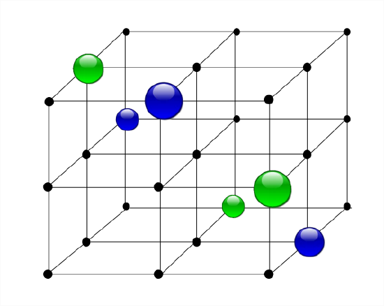
Illustrated in Figure 3.8, the array is mostly zeros, with three 1s and three -1s arranged antisymmetrically. The essential property of the alternating tensor is that it is completely antisymmetric, meaning that the interchange of any two indices results in a sign change. Two other properties follow from this one:
- Any element with two equal indices must be zero.
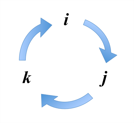
- Cyclic permutations of the indices have no effect. What is a cyclic permutation? The idea is illustrated in figure \(\PageIndex{2}\). For example, suppose we start with \(\epsilon_{ijk}\), then move the \(k\) back to the first, or leftmost position, shifting \(i\) and \(j\) to the right to make room, resulting in \(\epsilon{kij}\). That’s a cyclic permutation.
Examine Equation \(\ref{eq:12}\) and convince yourself that these two statements are true. See Appendix D for a proof that they have to be true.


The \(\varepsilon - \delta\) relation
The alternating tensor is related to the 2nd-order identity tensor in a very useful way:
\[\varepsilon_{i j k} \varepsilon_{k l m}=\delta_{i l} \delta_{j m}-\delta_{i m} \delta_{j l}.\label{eq:13} \]
For us, the main value of Equation \(\ref{eq:13}\) will be in deriving vector identities, as we will see below. Test your understanding of the \(\epsilon - \delta\) relation by completing exercise 17.
The cross product
The cross product is defined in terms of \(\underset{\sim}{\varepsilon}\) by
\[z_{k}=\varepsilon_{i j k} u_{i} v_{j}\label{eq:14} \]
You will sometimes see Equation \(\ref{eq:14}\) written with the free index in the first position: \(z_k = \epsilon_{kij}u_iv_j\). The two expressions are equivalent because \(kij\) is a cyclic permutation of \(ijk\) (see property 2 of \(\underset{\sim}{\varepsilon}\) listed above).
We will now list some essential properties of the cross product.
1. The cross product is anticommutative:
\[ \begin{align*}(\vec{v}\times\vec{u})_k &= \varepsilon_{ijk}v_iu_j \\ &= \varepsilon_{ijk}u_jv_i \;\; \text{(reordering)}\\ &= \varepsilon_{jik}u_iv_j \;\;\text{(relabeling i and j)}\\ &= -\varepsilon_{ijk}u_iv_j \;\;\text{(using antisymmetry)} \\ &= -(\vec{u}\times\vec{v})_k. \end{align*} \nonumber \]
2. The cross product is perpendicular to both \(\vec{u}\) and \(\vec{v}\). This is left for the reader to prove (exercise 18).
3. The magnitude of the cross product is
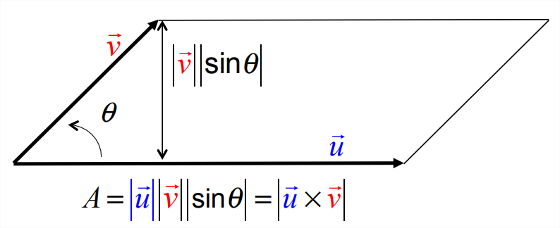
\[|\vec{z}|=|\vec{u}||\vec{v}||\sin \theta|,\label{eq:15} \]
where \(\theta\) is the angle between \(\vec{u}\) and \(\vec{v}\). This is easily proven by writing the squared magnitude of \(\vec{z}\) as
\[z_{k} z_{k}=\varepsilon_{i j k} u_{i} v_{j} \varepsilon_{k l m} u_{l} v_{m} \nonumber \]
then applying the \(\underset{\sim}{\varepsilon}-\underset{\sim}{\delta}\) relation. A geometric interpretation of Equation \(\ref{eq:15}\) is that the magnitude of the cross product is equal to the area of the parallelogram bounded by \(\vec{u}\) and \(\vec{v}\) (figure \(\PageIndex{4}\)).
Test your understanding of the cross product by completing exercise 18.
The determinant
The determinant of a \(3\times3\) matrix \(\underset{\sim}{A}\) can be written using \(\underset{\sim}{\varepsilon}\):
\[\operatorname{det}(\underset{\sim}{A})=\varepsilon_{i j k} A_{i 1} A_{j 2} A_{k 3},\label{eq:16} \]
where the columns are treated as vectors.5 The many useful properties of the determinant all follow from this definition (Appendix D).
1A counterexample to this is diagonality: a tensor can be diagonal in one coordinate system and not in others, e.g., exercise 10, or section 5.3.4. So diagonality is not an intrinsic property.
2up to a multiplicative constant
3This is true in Cartesian coordinates. In curved coordinate systems, e.g. Appendix I, the dot product is computed using a more general object called the metric tensor which we will not go into here.
4Tullio Levi-Civita (1873-1941) was an Italian mathematician. Among other things, he consulted with Einstein while the latter was developing the general theory of relativity.


