4.2: Flux and divergence
- Page ID
- 18061
The flux of a quantity is the rate at which it is transported across a surface, expressed as transport per unit surface area. A simple example is the volume flux, which we denote as \(Q\).
4.2.1 Volume flux through a rectilinear surface
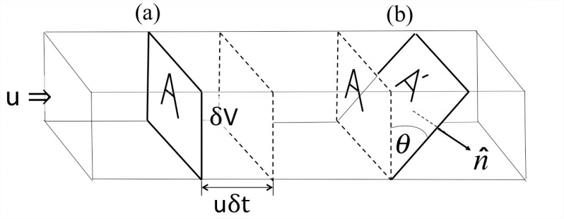
Consider the simple, rectilinear channel in (Figure \(\PageIndex{1}\)). The flow velocity \(\vec{u}\) is assumed to be uniform with magnitude \(|\vec{u}| = U\), and the cross-sectional area is A. After a time \(\delta t\), the flow through the cross-section marked (a) has travelled a distance \(U\delta t\) and occupies a volume \(\delta V = AU \delta t\). The volume flux is then
\[Q=\frac{\delta V}{\delta t}=A U \nonumber \]
Examples:
• A river 100 m wide and 2 m deep has cross-sectional area 200 m2. If we take the velocity to be 1 m s−1, then we estimate the volume flux as 200 m2×1 m s−1= 200 m3 s−1.
• The total volume flux of all of Earth’s rivers is \(\sim\) 106 m3 s−1.
• The Gulf Stream, a large ocean current that flows north along the east coast of the U.S., is typically 100 km wide and 1000 m deep, so the cross-sectional area is 108 m2. A typical velocity is 1 m s−1, so the corresponding volume flux is \(Q\) = 108 m3 s−1.
Oceanographers measure volume flux in units of Sverdrups1: 1 Sv = 106 m3 s−1. The world’s rivers therefore carry about 1 Sv., while the Gulf Stream carries 100 Sv.
Suppose now that the surface through which we calculate the volume flux is tilted at an angle \(\theta\) from the vertical (marked (b) in (Figure \(\PageIndex{1}\))). The volume flux is, of course, the same as that through the vertical section. The area of the vertical section is \(A^\prime \cos\theta\). We can therefore define the volume flux through a surface tilted at an arbitrary angle \(\theta\) from the vertical as \(Q = UA^\prime \cos\theta\). We can also express this flux in terms of the unit vector \(\hat{n}\), drawn normal to the surface \(A^\prime\). Note that the product \(U \cos\theta\) is equal to \(\vec{u}\cdot\hat{n}\).
4.2.2 Volume flux through a curved surface
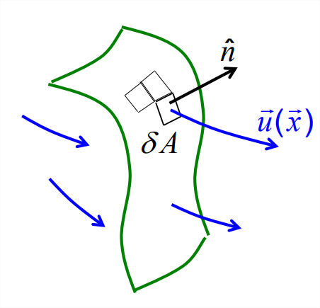
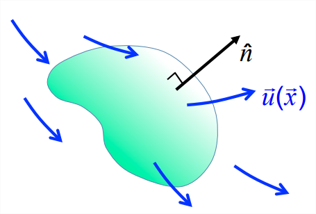
A curved surface can be thought of as being tiled by small, flat, surface elements with area \(\delta A\) and unit normal \(\hat{n}\). The tiling matches the surface exactly as the tile size shrinks to zero. The volume flux through each tile is \(\delta Q = \vec{u}\cdot\hat{n}\delta A\), just as in the case of the tilted surface in section 4.2.1. If we now sum over all of the tiles and take the limit as \(\delta A \rightarrow 0\), we obtain the general expression
4.2.3 Volume flux through an arbitrary closed surface: the divergence theorem
Flux through an infinitesimal cube
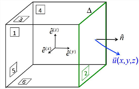
Consider a general velocity field \(\vec{u}\left(\vec{x}\right)=\left\{ u\left(\vec{x}\right), v\left(\vec{x}\right), w\left(\vec{x}\right)\right\}\), and somewhere within it a small, imaginary cube with edge dimension \(\Delta\) (Figure \(\PageIndex{4}\)). We would like to know the net volume flux out of the cube. We define a Cartesian coordinate system aligned with the cube as shown. We will now compute the outward volume flux across each of the faces, numbered 1-6 in the figure.
We begin with face #2, highlighted in green. On this face \(y = \frac{\Delta}{2}\), and the outward unit normal is \(\hat{n}=\hat{e}^{(y)}\). The volume flux may be written as
\[Q^{[2]}=\int_{[2]} \vec{u} \cdot \hat{n} d A=\int_{-\Delta / 2}^{\Delta / 2} d x \int_{-\Delta / 2}^{\Delta / 2} d z v(x, \Delta / 2, z).\label{eqn:2} \]
We now approximate the spatial variation of v by means of a first-order Taylor series expansion about the origin:
\[v(x, y, z)=v^{0}+v_{x}^{0} x+v_{y}^{0} y+v_{z}^{0} z+\ldots\label{eqn:3} \]
Here, subscripts indicate partial derivatives (for brevity) and the superscript “0” specifies evaluation at the origin. The dots at the end represent higher-order terms that will vanish later when we take the limit \(\Delta\rightarrow 0\); from here on we ignore these. Replacing the integrand in Equation \(\ref{eqn:2}\) with Equation \(\ref{eqn:3}\), we have
\[\begin{aligned}
Q^{[2]}=\int_{-\Delta / 2}^{\Delta / 2} d x \int_{-\Delta / 2}^{\Delta / 2} d z &\left[\quad v^{0}+v_{x}^{0} x+v_{y}^{0} \frac{\Delta}{2}+v_{z}^{0} z\right] \\
=&\left[\quad \Delta^{2} v^{0}+0+\Delta^{2} v_{y}^{0} \frac{\Delta}{2}+0\right] \\
=&\left(v^{0}+v_{y}^{0} \frac{\Delta}{2}\right) \Delta^{2}
\end{aligned} \nonumber \]
Now we repeat the process for the opposite face, #5. The only differences are that the uniform value of \(y\) becomes \(-\Delta/2\) and the outward normal becomes \(-\hat{e}^{(y)}\). The calculation therefore gives
\[Q^{[5]}=-\left(v^{0}-v_{y}^{0} \frac{\Delta}{2}\right) \Delta^{2} \nonumber \]
Summing the fluxes from faces 2 and 5 gives
\[Q^{[2]}+Q^{[5]}=2 \times v_{y}^{0} \frac{\Delta}{2} \Delta^{2}=v_{y}^{0} \Delta^{3}. \nonumber \]
Note that, if the velocity \(v\) were uniform, this net outward flux would be zero, i.e., what comes in one face goes out the other. The net flux is nonzero only when the velocities through the two faces differ. We can now repeat this process for each of the other two opposite pairs of faces:
\[Q^{[1]}+Q^{[4]}=u_{x}^{0} \Delta^{3}, \quad \text { and } \quad Q^{[3]}+Q^{[6]}=v_{z}^{0} \Delta^{3} \nonumber \]
Adding these results, we have the net outflow:
\[Q=\left(u_{x}^{0}+v_{y}^{0}+w_{z}^{0}\right) \Delta^{3} \nonumber \]
At this stage we take the limit as \(\Delta\rightarrow 0\) so that the higher-order terms that we have neglected vanish. Because our cube could have been placed anywhere in the velocity field, this result is true at every point and we don’t need drop the superscript “0”. The infinitesimal volume flux \(\delta Q\) from this small cube therefore expresses the divergence of the velocity field:
\[\delta Q=\vec{\nabla} \cdot \vec{u} \delta V,\label{eqn:4} \]
where \(\delta V\) is the limit of the volume \(\Delta^3\).
In many situations, the flows into and out of a small volume balance, and therefore \(\vec{\nabla}\cdot\vec{u}=0\). There are two exceptions:
1. There is a volume source, e.g., fluid is being pumped into the cube through a hose.
2. The fluid expands or contracts, e.g., as a result of heating or cooling.
Summing the cubes
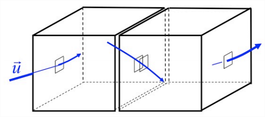
Suppose we now want to know the net outflow from two adjacent cubes. We would sum the flows through each face as before. Note, however, that the volume fluxes through the two adjacent faces exactly cancel. (The velocities are the same and the unit normals are opposite.) By Equation \(\ref{eqn:4}\), this net outflow equals the divergence evaluated at the center of each cube multiplied by the volume \(\delta V\) and summed over the two cubes.
We can generalize this to any assemblage of adjacent cubes: the net outflow is the sum of the outflows through the exterior faces only, because the flows through the interior faces cancel. Moreover, this is equal to the sum of the divergences in each cube times \(\delta V\).
The divergence theorem
An arbitrary volume can be approximated with arbitrary precision as an assemblage of small cubes. The foregoing results regarding the flux from a small cube, in the limit as \(\delta V \rightarrow 0\), give us the divergence theorem (also called Gauss’ theorem2):
Theorem: Within a given flow field \(\vec{u}\left(\vec{x}\right)\), imagine volume of space \(V\) bounded by an arbitrary closed surface \(A\). At each point on the surface, define the outward-pointing unit normal \(\hat{n}\). Then the net volume flux out the surface is given by the integral of its divergence throughout the volume:
\[Q=\oint_{A} \vec{u} \cdot \hat{n} d A=\int_{V} \vec{\nabla} \cdot \vec{u} d V,\label{eqn:5} \]
or, in index notation:
\[Q=\oint_{A} u_{i} n_{i} d A=\int_{V} \frac{\partial u_{i}}{\partial x_{i}} d V.\label{eqn:6} \]
In physical terms, the divergence theorem tells us that the flux out of a volume equals the sum of the sources minus the sinks within the volume.
The divergence theorem can be generalized considerably. First, \(\vec{u}\) does not have to be the flow velocity; the theorem holds for any vector field. Second, the theorem can be applied to higher-dimensional objects. Suppose, for example, that we take three separate vectors and concatenate them to form the columns of a matrix \(\underset{\sim}{A} \left(\vec{x}\right) = \left\{ \vec{u}\left(1\right),\vec{u}\left(2\right),\vec{u}\left( 3\right)\right\}\), or \(A_{ij} = u_i^{(j)}\). We can then concatenate Equation \(\ref{eqn:6}\) and find
\[\oint_{A} A_{i j} n_{i} d A=\int_{V} \frac{\partial A_{i j}}{\partial x_{i}} d V \quad \text { for } j=1,2,3\label{eqn:7} \]
One could also let the three vectors be the rows of \(\underset{\sim}{A}\), in which case the dummy index in Equation \(\ref{eqn:7}\) would be the second index of \(\underset{\sim}{A}\) instead of the first.3
1Harald Sverdrup (1888-1957) was a Norwegian oceanographer and meteorologist. He was the scientific director for the Amundsen expedition to the North pole, and was later director of the Scripps Institute of Oceanography in San Diego. He discovered the fundamental balance between wind and the Earth’s rotation that governs the large-scale ocean currents.
2Carl Friedrich Gauss (1777-1855) was a German mathematician and physicist. He is considered one of the greatest scientists in history, and it would be an insult to try to describe his accomplishments in a footnote. However, he did not actually discover the theorem that bears his name - it was used by Lagrange fifty years before Gauss found it.
3The derivation does not rely on \(\underset{\sim}{A}\) having the transformation properties of a Cartesian tensor. Indeed, if its columns transform as vectors, then it will not. Conversely, \(\underset{\sim}{A}\) may transform as a second-order tensor in which case its columns \(\vec{u}^{(1)}\) will not transform as vectors. The theorem works regardless.


