
11.9.2: Governing Equations
- Page ID
- 834

The energy balance on the control volume reads
\[
Q = C_p\, \left({T_0}_2 - {T_0}_1 \right)
\label{ray:eq:energy}
\]
\[
A\, ( P_1 - P_2 ) = \dot{m} \, ( V_2 - V_1)
\label{ray:eq:momentum}
\]
The mass conservation reads
\[
\rho_1 U_1 A = \rho_2 U_2 A = \dot{m}
\label{ray:eq:mass}
\]
Equation of state
\[
{P_1 \over \rho_1 \,T_1} =
{P_2 \over \rho_2 \,T_2}
\label{ray:eq:state}
\]
There are four equations with four unknowns, if the upstream conditions are known (or downstream conditions are known). Thus, a solution can be obtained. One can notice that equations (??), (??), and (??) are similar to the equations that were solved for the shock wave. Thus, results in the same as before (??)
Pressure Ratio
\[
\label{ray:eq:Pratio}
\dfrac{P_2 }{ P_1} =
\dfrac {1 + k\,{M_1}^{2} }{ 1 + k\,{M_2}^{2}}
\]
The equation of state (??) can further assist in obtaining the temperature ratio as
\[
\dfrac{T_2 }{ T_1} = \dfrac{P_2 }{ P_1} \dfrac{\rho_1 }{ \rho_2}
\label{ray:eq:Tratio}
\]
\[
\dfrac{\rho_1 }{ \rho_2} = \dfrac{U_2 }{ U_1} =
\dfrac{ \dfrac{U_2 }{ \sqrt{k\,R\,T_2} } \sqrt{k\,R\,T_2} }
{ \dfrac{U_1 }{ \sqrt{k\,R\,T_1} } \sqrt{k\,R\,T_1} }
= \dfrac{M_2 }{ M_1} \sqrt{ T_2 \over T_1}
\label{ray:eq:rhoR1}
\]
or in simple terms as
Density Ratio
\[
\label{ray:eq:rhoR}
\dfrac{\rho_1 }{ \rho_2} = \dfrac{U_2 }{ U_1} =
\dfrac{M_2 }{ M_1} \sqrt{\dfrac{ T_2 }{ T_1}}
\]
or substituting equations (??) and (??) into equation (??) yields
\[
{T_2 \over T_1} =
{1 + k\,{M_1}^{2} \over 1 + k\,{M_2}^{2}}\,
{M_2 \over M_1} \sqrt{ T_2 \over T_1}
\label{ray:eq:t2t1a}
\]
Temperature Ratio
\[
\label{ray:eq:t2t1b}
\dfrac{T_2 }{T_1} =
\left[ \dfrac{1 + k\,{M_1}^{2} }{ 1 + k\,{M_2}^{2}} \right]^{2}\,
\left(\dfrac{M_2 }{ M_1}\right)^{2}
\]
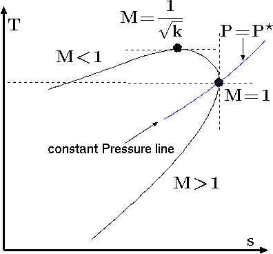
Fig. 11.40 The temperature entropy diagram for Rayleigh line.
The Rayleigh line exhibits two possible maximums one for \(dT/ds = 0 \) and for \(ds /dT =0\). The second maximum can be expressed as \(dT/ds = \infty\). The second law is used to find the expression for the derivative.
\[
{s_1 -s_2 \over C_p} = \ln {T_2 \over T_1}
- \dfrac{k -1 }{ k}\, \ln {P_2 \over P_1}
\label{ray:eq:2ndLaw}
\]
\[
\label{ray:eq:sndRlawEx}
\dfrac{s_1 -s_2 }{ C_p} =
2\, \ln \left[
{({1 + k\,{M_1}^{2}) \over (1 + k\,{M_2}^{2} ) } {M_2 \over M_1}}
\right] +
{k -1 \over k} \ln \left[
{1 + k\,{M21}^{2} \over 1 + k\,{M_1}^{2} } \right]
\qquad \,
\]
Let the initial condition \(M_1\), and \(s_1\) be constant and the variable parameters are \(M_2\), and \(s_2\). A derivative of equation (??) results in
\[
\dfrac{1 }{ C_p } \dfrac{ds }{ dM} =
\dfrac{2\, ( 1 - M^{2} ) }{ M\, (1 + k\,M^{2} )}
\label{ray:eq:sndRlawExDrivative}
\]
Taking the derivative of equation (??) and letting the variable parameters be \(T_2\), and \(M_2\) results in
\[
{dT \over dM} =
constant \times { 1 - k\,M^{2} \over \left( 1 + k\,M^2\right)^{3} }
\label{ray:eq:dTdM}
\]
\[
{dT \over ds} = constant \times
{M (1 - kM^2 ) \over ( 1 -M^2) ( 1 + kM^2 )^2 }
\label{ray:eq:dTds}
\]
On T–s diagram a family of curves can be drawn for a given constant. Yet for every curve, several observations can be generalized. The derivative is equal to zero when \(1 - kM^2 = 0\) or \(M = 1 /\sqrt{k}\) or when \(M \rightarrow 0\). The derivative is equal to infinity, \(dT/ds = \infty\) when \(M = 1\). From thermodynamics, increase of heating results in increase of entropy. And cooling results in reduction of entropy. Hence, when cooling is applied to a tube the velocity decreases and when heating is applied the velocity increases. At peculiar point of \(M = 1/\sqrt{k}\) when additional heat is applied the temperature decreases. The derivative is negative, \(dT/ds < 0\), yet note this point is not the choking point. The choking occurs only when \(M= 1\) because it violates the second law. The transition to supersonic flow occurs when the area changes, somewhat similarly to Fanno flow. Yet, choking can be explained by the fact that increase of energy must be accompanied by increase of entropy. But the entropy of supersonic flow is lower (Figure 11.40) and therefore it is not possible (the maximum entropy at \(M=1\).). It is convenient to refer to the value of \(M=1\).
The equation (??) can be written between choking point and any point on the curve.
Pressure Ratio
\[
\label{ray:eq:Pratioa}
\dfrac{P^{*} }{ P_1} = {1 + k\,{M_1}^{2} \over 1 + k}
\]
The temperature ratio is
Pressure Ratio
\[
\label {ray:eq:Tratioa}
{T^{*} \over T_1} = {1 \over M^2}
\left( {1 + k{M_1}^{2} \over 1 + k} \right)^{2}
\]
The stagnation temperature can be expressed as
\[
Callstack:
    at (Bookshelves/Civil_Engineering/Book:_Fluid_Mechanics_(Bar-Meir)/11:_Compressible_Flow_One_Dimensional/11.9:_Rayleigh_Flow/11.9.2:_Governing_Equations), /content/body/p[23]/span, line 1, column 4
{T_1 \left( 1 + \dfrac{k -1 }{ 2} {M_1}^{2} \right)
\over T^{*} \left( \dfrac{1 + k } {2} \right)}
\label{ray:eq:T0ratio2}
\] or explicitly
Stagnation Temperature Ratio
\[
\label{ray:eq:T0ratio}
Callstack:
    at (Bookshelves/Civil_Engineering/Book:_Fluid_Mechanics_(Bar-Meir)/11:_Compressible_Flow_One_Dimensional/11.9:_Rayleigh_Flow/11.9.2:_Governing_Equations), /content/body/div[6]/p[2]/span, line 1, column 4
\dfrac{ 2\, ( 1 + k )\, {M_1}^{2} }{ (1 + k\,M^{2})^2}
\left( 1 + {k -1 \over 2} {M_1} ^2 \right)
\]
The stagnation pressure ratio reads
\[ \dfrac
Callstack:
    at (Bookshelves/Civil_Engineering/Book:_Fluid_Mechanics_(Bar-Meir)/11:_Compressible_Flow_One_Dimensional/11.9:_Rayleigh_Flow/11.9.2:_Governing_Equations), /content/body/p[25]/span, line 1, column 4
{P_1 \left( 1 + \dfrac{k -1 }{ 2}\, {M_1}^{2} \right)
\over P^{*} \left( {1 + k } \over 2 \right)}
\label{ray:eq:P0ratio2}
\] or explicitly
Stagnation Pressure Ratio
\[
\label{ray:eq:P0ratio}
\dfrac
Callstack:
    at (Bookshelves/Civil_Engineering/Book:_Fluid_Mechanics_(Bar-Meir)/11:_Compressible_Flow_One_Dimensional/11.9:_Rayleigh_Flow/11.9.2:_Governing_Equations), /content/body/div[7]/p[2]/span, line 1, column 4
{\left({ 1 + k \over 1 + k\,{M_1}^2}\right)}
\left( { 1 + k\,{M_1}^2 \over {(1 + k) \over 2}} \right)^{\dfrac{k }{ k -1}}
\]
Contributors and Attributions
Dr. Genick Bar-Meir. Permission is granted to copy, distribute and/or modify this document under the terms of the GNU Free Documentation License, Version 1.2 or later or Potto license.