6.21: The Doron et al. (1987) and Doron and Barnea (1993) Model

6.21.1 The 2 Layer Model (2LM)

Doron et al. (1987) and Doron & Barnea (1993) developed a 2 layer model (2LM) in 1987 and extended it to a 3 layer model (3LM) in 1993. Some elements of the models are similar to the Wilson-GIW (1979) model, other elements are different. In the description of the model the symbols of this book are used.

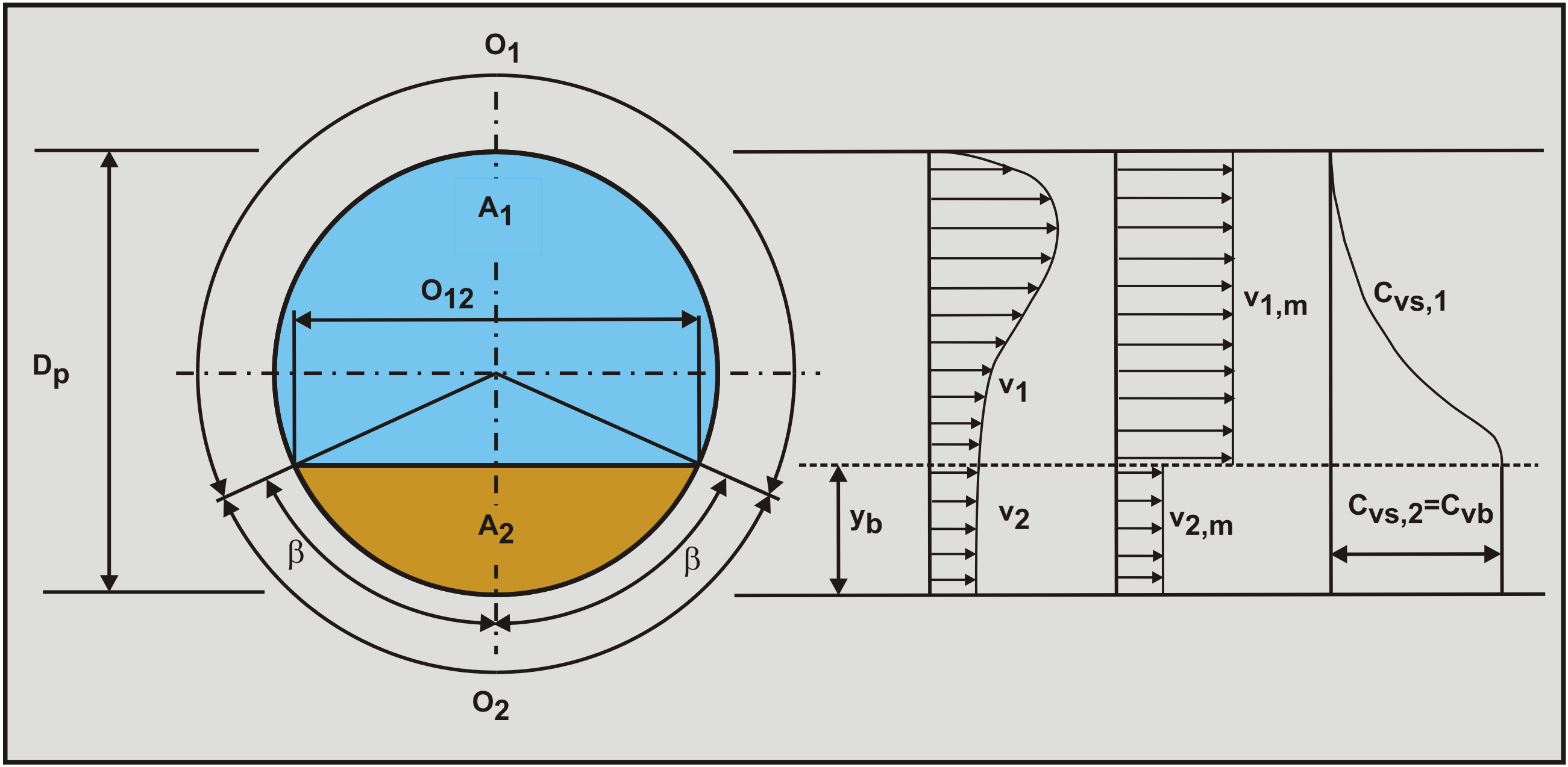
Now consider a pipe with diameter D_p and cross section A_p, see Figure 6.20-1. Suppose the bottom part of the pipe is filled with a stationary or sliding bed with a bed concentration C_vb and above the bed there is heterogeneous transport. 3 indices are used, the index 1 (original h) for the heterogeneous transport, the index 2 (original b) for the bed and the index 12 (original i) for the interface between the bed and the heterogeneous transport. A coordinate system is used starting at the bottom of the pipe with coordinate y where the bed height is y₁₂ (original y_b). The cross section of the heterogeneous flow is A₁ (original A_h). The cross section of the bed is A₂ (original A_b). The length of the wetted circumference of the heterogeneous flow is O₁ (original S_h). The length of the circumference between the bed and the pipe wall is O₂ (original S_b). The length of the interface between the heterogeneous flow and the bed is O₁₂ (original S_i). The angle starting at the vertical and ending at the top of the bed y₁₂ is named β.The velocity in the heterogeneous cross section is v₁ (original U_h). The velocity of the bed is v₂ (original U_b). The cross section averaged velocity or line speed is v_ls (original U_s).

Figure 6.21-1: The 2 layer model with suspension in the upper layer.

For the solids phase the continuity equation yields, neglecting slip between the two phases:

\[\ \mathrm{v}_{\mathrm{1}} \cdot \mathrm{A}_{\mathrm{1}} \cdot \mathrm{C}_{\mathrm{v s}, \mathrm{1}}+\mathrm{v}_{\mathrm{2}} \cdot \mathrm{A}_{\mathrm{2}} \cdot \mathrm{C}_{\mathrm{v b}}=\mathrm{v}_{\mathrm{l} \mathrm{s}} \cdot \mathrm{A}_{\mathrm{p}} \cdot \mathrm{C}_{\mathrm{v} \mathrm{t}}\]

For the liquid phase the continuity equation yields, neglecting slip between the two phases:

\[\ \mathrm{v}_{1} \cdot \mathrm{A}_{1} \cdot\left(1-\mathrm{C}_{\mathrm{v s}, 1}\right)+\mathrm{v}_{2} \cdot \mathrm{A}_{2} \cdot\left(1-\mathrm{C}_{\mathrm{v b}}\right)=\mathrm{v}_{\mathrm{l s}} \cdot \mathrm{A}_{\mathrm{p}} \cdot\left(1-\mathrm{C}_{\mathrm{v t}}\right)\]

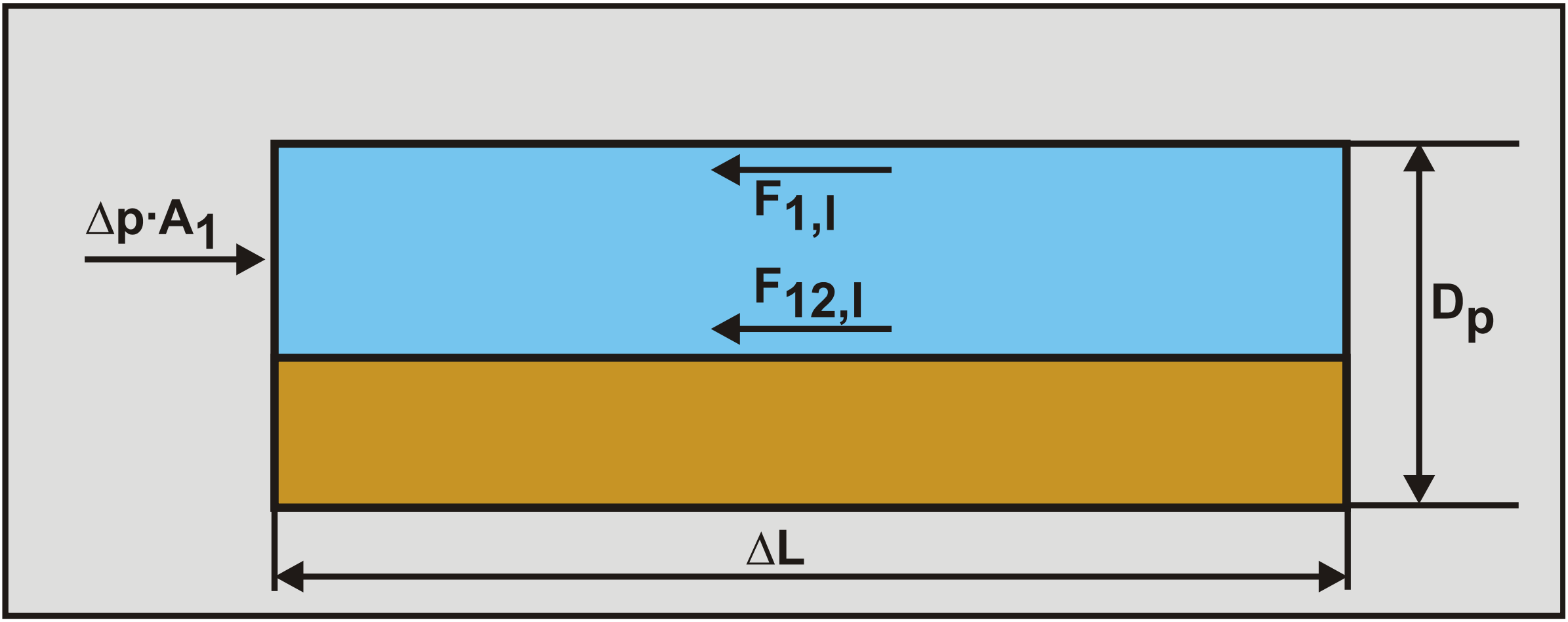
The force balance on the heterogeneous layer yields:

\[\ \mathrm{-A_{1} \cdot \Delta p=F_{1,\mathrm{l}}+F_{12,\mathrm{l}} \quad\text{ and }\quad-A_{1} \cdot \frac{\Delta p}{\Delta L}=\tau_{1,\mathrm{l}} \cdot O_{1}+\tau_{12,\mathrm{l}} \cdot O_{12}}\]

The first term on the right hand side is the Darcy Weisbach friction between the liquid and the pipe wall, the second term the Darcy Weisbach friction between the liquid and the bed.

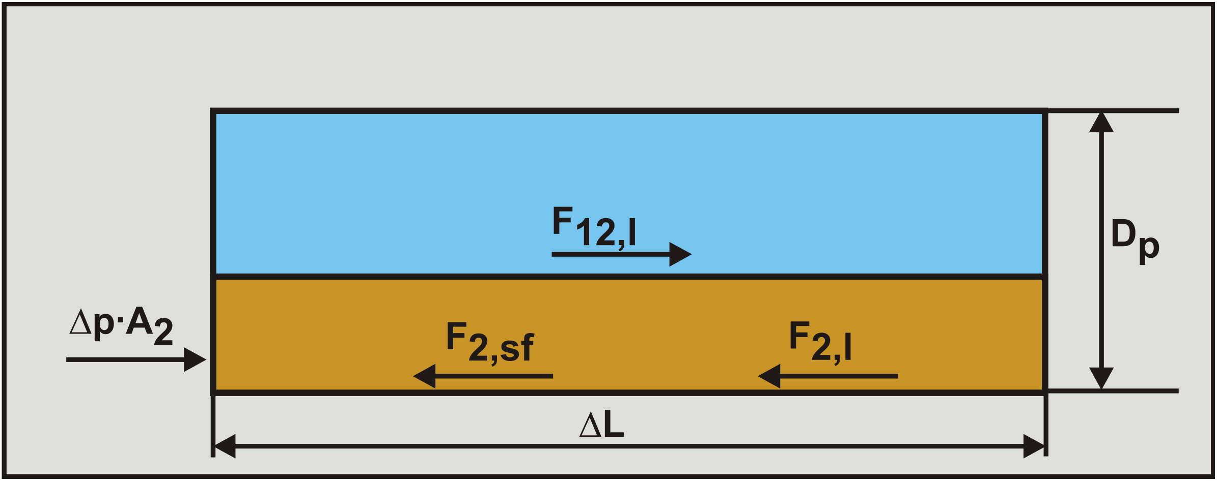
The force balance on the bed layer yields:

\[\ \mathrm{-A_{2} \cdot \Delta p+F_{12,\mathrm{l}}=F_{2, \mathrm{sf}}+F_{2,\mathrm{l}} \quad\text{ and }\quad-A_{2} \cdot \frac{\Delta p}{\Delta L}+\tau_{12,\mathrm{l}} \cdot O_{12}=\tau_{2, \mathrm{sf}} \cdot O_{2}+\tau_{2,\mathrm{l}} \cdot O_{2}}\]

Because the term Δp/ΔL, the pressure gradient, is negative, a minus sign is added in front. The first term on the right hand side is the sliding friction between the bed and the pipe wall, the second term is the Darcy Weisbach friction of the pore water with the pipe wall. In the case of a sliding bed, the sliding friction force is a constant, but in case of a fixed bed this force will have a value between zero and the sliding friction force. The normal force between the bed and the pipe wall, necessary to calculate the sliding friction force, consists of two components. The first component is based on the submerged weight of the solid particles in the bed, while the second component is based on the transmission of normal stresses at the heterogeneous-bed interface, resulting in a shear force at the interface. This gives for the normal force F_N1 resulting from the submerged weight:

\[\ \mathrm{F}_{\mathrm{N} 1}=\rho_{\mathrm{l}} \cdot \mathrm{g} \cdot \Delta \mathrm{L} \cdot \mathrm{R}_{\mathrm{s d}} \cdot \mathrm{C}_{\mathrm{v b}} \cdot \frac{\mathrm{D}_{\mathrm{p}}^{2}}{\mathrm{2}} \cdot(\sin (\beta)-\boldsymbol{\beta} \cdot \cos (\boldsymbol{\beta}))\]

This gives for the normal force F_N1 in the Doron notation:

\[\ \mathrm{F}_{\mathrm{N} 1}=\rho_{\mathrm{l}} \cdot \mathrm{g} \cdot \Delta \mathrm{L} \cdot \mathrm{R}_{\mathrm{s d}} \cdot \mathrm{C}_{\mathrm{v b}} \cdot \frac{\mathrm{D}_{\mathrm{p}}^{2}}{\mathrm{2}} \cdot\left(\left(\frac{\mathrm{2} \cdot \mathrm{y}_{\mathrm{b}}}{\mathrm{D}_{\mathrm{p}}}-\mathrm{1}\right) \cdot \beta+\sin (\beta)\right)\]

Figure 6.21-2: The forces on the liquid above the bed.

Figure 6.21-3: The forces on the bed.

The normal force is determined using the Wilson (1970) hydrostatic pressure approach. There may be an additional normal force on the bed resulting from the submerged weight of the particles above this bed level. The additional normal force due to transmission of stress from the interface through bed particles is, after Bagnold (1954) and (1957):

\[\ \mathrm{F}_{\mathrm{N} 2}=\frac{\tau_{12} \cdot \mathrm{O}_{12} \cdot \Delta \mathrm{L}}{\tan (\varphi)}\]

With φ the angle of internal friction at the top of the bed with values of 20° to 40°. The total normal force F_N between the bed and the pipe wall is now:

\[\ \mathrm{F}_{\mathrm{N}}=\mathrm{F}_{\mathrm{N} 1}+\mathrm{F}_{\mathrm{N} 2}=\rho_{\mathrm{l}} \cdot \mathrm{g} \cdot \Delta \mathrm{L} \cdot \mathrm{R}_{\mathrm{s} \mathrm{d}} \cdot \mathrm{C}_{\mathrm{v} \mathrm{b}} \cdot \frac{\mathrm{D}_{\mathrm{p}}^{2}}{\mathrm{2}} \cdot\left(\left(\frac{\mathrm{2} \cdot \mathrm{y}_{\mathrm{b}}}{\mathrm{D}_{\mathrm{p}}}-\mathrm{1}\right) \cdot \beta+\sin (\beta)\right)+\frac{\tau_{12} \cdot \mathrm{O}_{12} \cdot \Delta \mathrm{L}}{\tan (\varphi)}\]

Giving for the sliding friction force F_2,sf between the bed and the pipe wall in case of a sliding bed:

\[\ \mathrm{F}_{2, \mathrm{sf}}=\mu_{\mathrm{sf}} \cdot\left(\rho_{\mathrm{l}} \cdot \mathrm{g} \cdot \Delta \mathrm{L} \cdot \mathrm{R}_{\mathrm{sd}} \cdot \mathrm{C}_{\mathrm{vb}} \cdot \frac{\mathrm{D}_{\mathrm{p}}^{2}}{2} \cdot\left(\left(\frac{\mathrm{2} \cdot \mathrm{y}_{\mathrm{b}}}{\mathrm{D}_{\mathrm{p}}}-\mathrm{1}\right) \cdot \beta+\sin (\beta)\right)+\frac{\tau_{12} \cdot \mathrm{O}_{12} \cdot \Delta \mathrm{L}}{\tan (\varphi)}\right)\]

The hydrodynamic resistance force F_1,l between the liquid in the bed and the pipe wall will only occur if the bed is sliding, this force can be determined by:

\[\ \mathrm{F}_{\mathrm{1}, \mathrm{l}}=\tau_{\mathrm{1}, \mathrm{l}} \cdot \mathrm{O}_{\mathrm{1}} \cdot \Delta \mathrm{L} \quad\text{ and }\quad \mathrm{F}_{\mathrm{2}, \mathrm{1}}=\tau_{\mathrm{2}, \mathrm{l}} \cdot \mathrm{O}_{\mathrm{2}} \cdot \Delta \mathrm{L}\]

The hydrodynamic shear stresses may be expressed by:

\[\ \mathrm{\tau_{1,l}=\frac{F_{1,l}}{O_{1} \cdot \Delta L}=\frac{\lambda_{l}}{8} \cdot \rho_{1} \cdot v_{1}^{2} \quad\text{ and }\quad \tau_{2,l}=\frac{F_{2,l}}{O_{2} \cdot \Delta L}=\frac{\lambda_{2,l}}{8} \cdot \rho_{2} \cdot v_{2}^{2}}\]

The Darcy Weisbach friction coefficients are evaluated from:

\[\ \frac{\lambda_{1}}{4}=\alpha_{1} \cdot\left(\frac{\mathrm{v}_{1} \cdot \mathrm{D}_{\mathrm{H} 1}}{v_{1}}\right)^{-\beta_{1}}\quad\text{ and }\quad\frac{\lambda_{2,1}}{4}=\alpha_{2} \cdot\left(\frac{\mathrm{v}_{2} \cdot \mathrm{D}_{\mathrm{H} 2}}{v_{2}}\right)^{-\beta_{2}}\]

The hydraulic diameters of cross sections 1 and 2 can be determined with:

\[\ \mathrm{D}_{\mathrm{H} 1}=\frac{4 \cdot \mathrm{A}_{1}}{\mathrm{O}_{1}+\mathrm{O}_{12}} \quad\text{ and }\quad \mathrm{D}_{\mathrm{H} 2}=\frac{4 \cdot \mathrm{A}_{2}}{\mathrm{O}_{2}+\mathrm{O}_{12}}\]

The viscosities \(\ v_{ \mathrm{1}}\) and \(\ v_{ \mathrm{2}}\) are the mean viscosities of the liquid in the two layers and should be taken equal to the liquid viscosity \(\ v_{ \mathrm{1}}\), unless the particles are very small influencing the viscosity. The coefficients α1 and α2 were taken 0.046 and the powers β1 and β2 both 0.2, for turbulent flow which is normally the case. The interfacial shear stress is expressed in terms of the relative velocity between the two layers.

\[\ \tau_{12,\mathrm{l}}=\frac{\lambda_{12}}{8} \cdot \rho_{12} \cdot\left(\mathrm{v_{1}-v_{2}}\right)^{2} \quad\text{ and }\quad \mathrm{F_{12,\mathrm{l}}=\tau_{12,\mathrm{l}} \cdot O_{12} \cdot \Delta L}\]

The Darcy Weisbach friction coefficient associated with the interface is evaluated using the Colebrook & White (1937) equation, with the particle diameter for the roughness. According to Televantos et al. (1979) the resulting Darcy Weisbach friction factor should be multiplied by 2, taking into account the effects of particle collisions, as well as entrainment and deposition of particles at the interface, which tend to increase the interfacial friction coefficient.

\[\ \lambda_{12}=\frac{2 \cdot 1.325}{\left(\ln \left(\frac{\mathrm{d}}{3.7 \cdot \mathrm{D}_{\mathrm{H} 1}}+\frac{2.51}{\mathrm{Re}_{\mathrm{H} 1} \cdot \sqrt{\lambda_{12}}}\right)\right)^{2}}\quad\text{ or }\quad\lambda_{12}=\frac{2 \cdot 1.325}{\left(\ln \left(\frac{\mathrm{d}}{3.7 \cdot \mathrm{D}_{\mathrm{H} 1}}+\frac{5.75}{\mathrm{Re}_{\mathrm{H} 1} 0.9}\right)\right)^{2}}\]

The densities of the two layers are calculated according to:

\[\ \begin{array}{left} \rho_{1}=\rho_{\mathrm{s}} \cdot \mathrm{C}_{\mathrm{vs}, 1}+\rho_{\mathrm{l}} \cdot\left(1-\mathrm{C}_{\mathrm{vs}, 1}\right)\\
\rho_{2}=\rho_{\mathrm{s}} \cdot \mathrm{C}_{\mathrm{vb}}+\rho_{\mathrm{l}} \cdot\left(1-\mathrm{C}_{\mathrm{vb}}\right)\end{array}\]

The bed concentration is assumed to be 52%. The viscosity of the mixture is considered equal to the viscosity of the carrier liquid. The particles used are coarse and much larger than the scale of the viscous sub layer, hence they do not affect the apparent viscosity.

The conservation equations deal with the horizontal direction of a horizontal pipe. In the vertical direction of a cross section of the pipe however a dispersion mechanism of the solid particles in the upper layer should be taken into account. This is assumed to be a turbulent diffusion process, which is governed by large scale eddies and tends to make the flow isotropic. It is the cause of a motion of particles from a high concentration zone to a low concentration zone, moving particles upwards. This tendency is balanced at steady state by gravity resulting in the settling of particles on top of the bed. This mechanism is represented by the well-known diffusion equation:

\[\ \varepsilon^{\prime} \cdot \frac{\partial^{2} \mathrm{C}(\mathrm{y})}{\partial \mathrm{y}^{2}}+\mathrm{v}_{\mathrm{t}}^{\prime} \cdot \frac{\partial \mathrm{C}(\mathrm{y})}{\partial \mathrm{y}}\]

Assuming that the concentration only depends on the vertical position and assuming a mean diffusion coefficient and terminal settling velocity, the concentration can be obtained by integrating the above equation twice, giving:

\[\ \left.\mathrm{C}(\mathrm{y})=\mathrm{C}_{\mathrm{v b}} \cdot \mathrm{e}^{\left(-\frac{\mathrm{v}_{\mathrm{t h}}}{\varepsilon} \cdot\left(\mathrm{y}-\mathrm{y}_{12}\right)\right.}\right)\]

Now assuming a mean cross flow diffusion coefficient of:

\[\ \varepsilon=0.052 \cdot \mathrm{u}_{*} \cdot \mathrm{R} \quad\text{ with: }\quad \mathrm{u}_{*}=\sqrt{\frac{\lambda_{1}}{\mathrm{8}}} \cdot \mathrm{v}_{1}\]

Solves the concentration distribution above the bed. The terminal settling velocity can be determined by, for example, the Ruby & Zanke (1977) equation (4.4-5).

\[\ \mathrm{v}_{\mathrm{t}}=\frac{\mathrm{1 0} \cdot v_{\mathrm{l}}}{\mathrm{d}} \cdot(\sqrt{1+\frac{\mathrm{R}_{\mathrm{s d}} \cdot \mathrm{g} \cdot \mathrm{d}^{\mathrm{3}}}{\mathrm{1 0 0} \cdot v_{\mathrm{l}}^{\mathrm{2}}}}-\mathrm{1})\]

For a cluster of particles the Richardson and Zaki (1954) equation (4.6-1) can be applied.

\[\ \frac{\mathrm{v}_{\mathrm{t h}}}{\mathrm{v}_{\mathrm{t}}}=\left(1-\mathrm{C}_{\mathrm{v s}}\right)^{\beta}\]

Integration of the above equation gives the mean concentration in the upper dispersed layer:

\[\ \left.\mathrm{C}_{\mathrm{v} \mathrm{s}, \mathrm{1}}=\frac{\mathrm{C}_{\mathrm{v} \mathrm{b}} \cdot \mathrm{D}_{\mathrm{p}}^{2}}{\mathrm{2} \cdot \mathrm{A}_{\mathrm{1}}} \cdot \int_{\beta_{12}}^{\pi} \mathrm{e}^{\left(-\frac{\mathrm{v}_{\mathrm{t h}} .}{\varepsilon} \cdot \frac{\mathrm{D}_{\mathrm{p}}}{2} \cdot\left(\cos \left(\beta_{12}\right)-\cos (\beta)\right)\right.}\right) \cdot \sin ^{2}(\beta) \cdot \mathrm{d} \beta\]

Equations (6.21-1), (6.21-2), (6.21-3), (6.21-4) and the above equation can be solved for any set of operational conditions for the following 5 unknowns: The mean velocity in the dispersed layer, the mean velocity of the bed, the mean concentration in the dispersed layer, the bed height or angle and the pressure gradient.

Three special cases will be considered, fully suspended flow, flow with a stationary bed and flow with a sliding bed.

Flow with a stationary bed:

In this case the bed velocity equals zero, reducing the number of equations. The sliding friction however is no longer defined. This gives:

\[\ \mathrm{C}_{\mathrm{v t}, \mathrm{1}}=\mathrm{C}_{\mathrm{v s}, \mathrm{1}}=\mathrm{C}_{\mathrm{v t}} \quad\text{ and }\quad \mathrm{v}_{\mathrm{1}}=\mathrm{v}_{\mathrm{l} \mathrm{s}} \cdot \frac{\mathrm{A}_{\mathrm{p}}}{\mathrm{A}_{\mathrm{1}}} \quad\text{ and }\quad \mathrm{v}_{2}=\mathrm{0}\]

Since the average concentration above the bed C_vt is known, the bed height y_b or bed angle β can be determined by iteration from:

\[\ \mathrm{ C_{v t}=\frac{C_{v b} \cdot D_{p}^{2}}{2 \cdot A_{1}} \cdot \int_{\beta_{12}}^{\pi} e^{\left(-\frac{v_{t h}}{\varepsilon} \cdot \frac{D_{p}}{2} \cdot\left(\cos \left(\beta_{12}\right)-\cos (\beta)\right)\right)} \cdot \sin ^{2}(\beta) \cdot d \beta}\]

Once the bed angle β is determined, all unknowns can be solved, also resulting in the pressure gradient. The static friction force follows from equation (6.21-4). As long as the static friction force is smaller than the sliding friction force, the bed is stationary. As soon as the static friction force found here is larger than the sliding friction force, the bed is sliding and the sliding bed methodology should be used. This was first presented by Wilson (1970)

Flow with a moving bed:

The whole set of equations (6.21-1), (6.21-2), (6.21-3), (6.21-4) and (6.21-22) has to be solved. The concentration profile can be determined with equation (6.21-18).

Fully suspended flow:

When the bed height approaches zero, transition to fully suspended flow occurs. This transition may also occur directly from the stationary bed regime, if the shear stress on the bed is never high enough to make the bed sliding. The pressure gradient can now be determined with:

\[\ \begin{array}{left} -\frac{\Delta \mathrm{p}}{\Delta \mathrm{L}}=\lambda_{1} \cdot \frac{1}{2} \cdot \rho_{\mathrm{m}} \cdot \mathrm{v}_{\mathrm{l} \mathrm{s}}^{2}\\
\rho_{\mathrm{m}}=\rho_{\mathrm{l}} \cdot\left(1-\mathrm{C}_{\mathrm{v} \mathrm{s}}\right)+\rho_{\mathrm{s}} \cdot \mathrm{C}_{\mathrm{v} \mathrm{s}}\end{array}\]

The no slip condition is still used here, assuming spatial and delivered volumetric concentrations are equal. This is very doubtful at the transition from a bed to full suspended flow. The vertical concentration profile can now be determined with:

\[\ \mathrm{C}(\mathrm{y})=\mathrm{C}_{\mathrm{v B}} \cdot \mathrm{e}^{\left(-\frac{\mathrm{v}_{\mathrm{t h}}}{\varepsilon} \cdot \mathrm{y}\right)}\]

The concentration at the bottom of the pipe C_vB is not equal to the bed concentration C_vb, but will have a lower value. Since the volumetric concentration of the suspension is known, the concentration at the bottom of the pipe can be determined with:

\[\ \mathrm{ \left.C_{v t}=\frac{C_{v B} \cdot D_{p}^{2}}{2 \cdot A_{p}} \cdot \int_{0}^{\pi} e^{\left(-\frac{v_{t h}}{\varepsilon} \cdot \frac{D_{p}}{2} \cdot(1-\cos (\beta))\right.}\right) \cdot \sin ^{2}(\beta) \cdot d \beta=\frac{2 \cdot C_{v B}}{\pi} \cdot \int_{0}^{\pi} e^{\left(-\frac{v_{t h}}{\varepsilon} \cdot \frac{D_{p}}{2} \cdot(1-\cos (\beta))\right)} \cdot \sin ^{2}(\beta) \cdot d \beta}\]

Or according to Doron et al. (1987):

\[\ \mathrm{C_{v B}=\frac{\pi}{2} \cdot C_{v t} \cdot \int_{0}^{\pi} e^{\left(-\frac{v_{t h}}{\varepsilon} \cdot \frac{D_{p}}{2} \cdot(1-\cos (\beta))\right)} \cdot \sin ^{2}(\beta) \cdot d \beta}\]

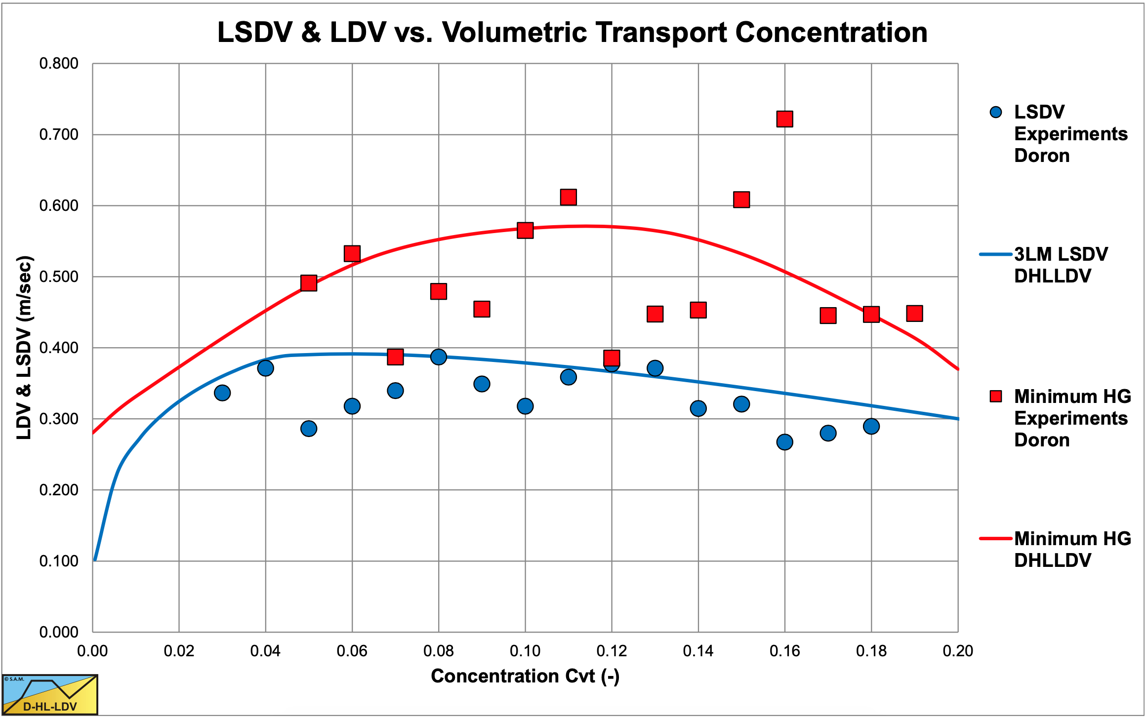
Doron et al. (1987) carried out experiments with an 11 m long Plexiglas pipe with an internal diameter of 51 mm (2 inch). They used black Acetal with a density of 1.24 tons/m, a diameter of 3 mm, a sliding friction coefficient of 0.3 and tan(φ)=0.6. Figure 6.21-8, Figure 6.21-11 and Figure 6.21-14 show some of the hydraulic gradient experimental data in a relative excess hydraulic gradient versus the liquid hydraulic gradient graph, while Figure 6.21-6 shows the observed Limit of Stationary Deposit Velocity (LSDV) and the Minimum Hydraulic Gradient Velocity (MHGV) versus the DHLLDV Framework, giving a good correlation. Figure 6.21-7 shows bed height data of Harada et al. (1989) versus the DHLLDV Framework, also giving a good correlation.

6.21.2 The 3 Layer Model (3LM)

The main limitation of the Doron et al. (1987) 2 layer model is its inability to predict accurately enough the existence of a stationary bed at low line speeds (flow rates). There are cases where a stationary bed was observed, yet the model predicts a moving bed. For dredging practice this is not really important, since dredging practice will not operate in this region of flow rates. However in order to understand the process of slurry flow in all aspects Doron & Barnea (1993) developed a 3 layer model. For high flow rates they still use the 2 layer model, but for low flow rates it is assumed that the bed consists of 2 layers, a stationary layer at the bottom of the pipe and a moving layer above it. The upper portion of the pipe is still occupied with a heterogeneous mixture. The forces on particles at the top of the bed are determined from a moment balance with the drag force giving the driving moment and the submerged weight giving the resisting moment. The derivation is similar to the derivation of the Shields curve in Chapter 5 and will not be discussed here. The 3 layer model gives a lower hydraulic gradient at very low flow rates compared to the 2 layer model, however the experimental data do not confirm the one or the other. Only the observation of a stationary bed at low flow rates would be in favor of the 3 layer model.

Figure 6.21-4: The 3 layer model with suspension in the upper layer and a stationary bed in the lowest layer.

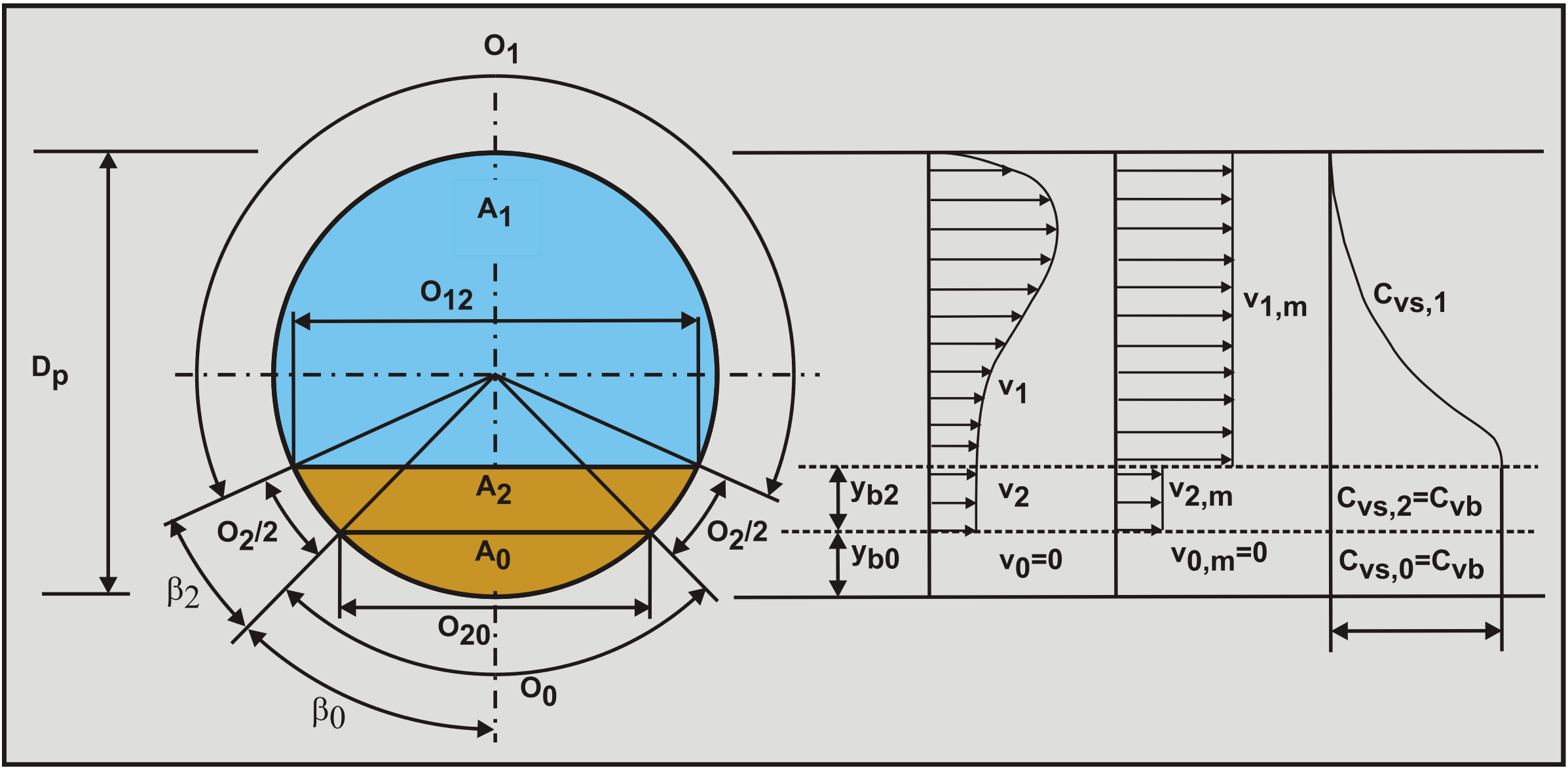
Figure 6.21-4 shows the heterogeneous upper layer A₁, the moving bed intermediate layer A₂ and the stationary bed lowest layer A₀. The velocity v₂ and the thickness y_b2 of the moving bed are related based on the equilibrium of moments on a particle, based on cubic packing with C_vb=0.52. This relation is:

\[\ \mathrm{v}_{2}=\sqrt{\frac{\mathrm{0 . 7 7 9} \cdot \mathrm{R}_{\mathrm{s d}} \cdot \mathrm{g} \cdot \mathrm{d}}{\mathrm{C}_{\mathrm{D}}} \cdot\left(\mathrm{C}_{\mathrm{v b}} \cdot \frac{\mathrm{y}_{\mathrm{b} 2}}{\mathrm{d}}+\left(\mathrm{1}-\mathrm{C}_{\mathrm{v b}}\right)\right)}\]

So the higher the velocity of the moving bed, the thicker the moving bed, until the thickness of the stationary bed is zero and the 2LM has to be applied. Note that it is assumed that the moving bed concentration is assumed to be constant and equal to 0.52 and that the circular shape of the pipe is not taken into account here.

For the solids phase the continuity equation yields, neglecting slip between the two phases:

\[\ \mathrm{v}_{\mathrm{1}} \cdot \mathrm{A}_{\mathrm{1}} \cdot \mathrm{C}_{\mathrm{v s}, \mathrm{1}}+\mathrm{v}_{\mathrm{2}} \cdot \mathrm{A}_{\mathrm{2}} \cdot \mathrm{C}_{\mathrm{v b}}=\mathrm{v}_{\mathrm{l} \mathrm{s}} \cdot \mathrm{A}_{\mathrm{p}} \cdot \mathrm{C}_{\mathrm{v} \mathrm{t}}\]

For the liquid phase the continuity equation yields, neglecting slip between the two phases:

\[\ \mathrm{v}_{1} \cdot \mathrm{A}_{1} \cdot\left(1-\mathrm{C}_{\mathrm{v s}, 1}\right)+\mathrm{v}_{2} \cdot \mathrm{A}_{2} \cdot\left(1-\mathrm{C}_{\mathrm{v} \mathrm{b}}\right)=\mathrm{v}_{\mathrm{l} \mathrm{s}} \cdot \mathrm{A}_{\mathrm{p}} \cdot\left(1-\mathrm{C}_{\mathrm{v t}}\right)\]

Figure 6.21-5: The forces on the moving bed and the stationary bed.

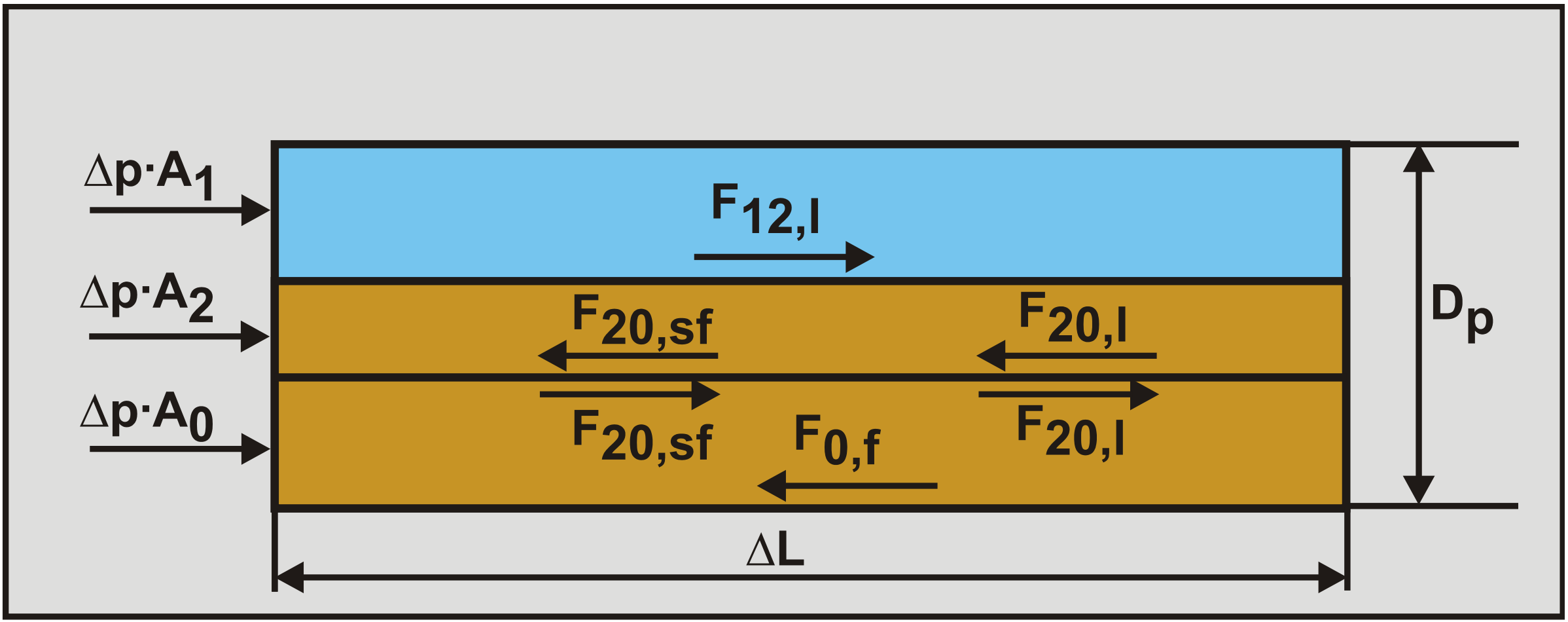
The force balance on the heterogeneous layer yields, see Figure 6.21-2, similar to the 2LM model:

\[\ \mathrm{ -A_{1} \cdot \Delta p=F_{1,\mathrm{l}}+F_{12,\mathrm{l}} \quad\text{ and }\quad-A_{1} \cdot \frac{\Delta p}{\Delta L}=\tau_{1,\mathrm{l}} \cdot O_{1}+\tau_{12,\mathrm{l}} \cdot O_{12}}\]

These forces consist of the driving force due to the pressure gradient on the left hand side and the resisting forces due to Darcy Weisbach friction between the liquid with the pipe wall and the liquid with the bed. The force balance on the moving bed layer yields:

\[\ \begin{array}{left}-\mathrm{A}_{2} \cdot \Delta \mathrm{p}+\mathrm{F}_{12,\mathrm{l}}=\mathrm{F}_{20, \mathrm{sf}}+\mathrm{F}_{\mathrm{2 0}, \mathrm{l}}+\mathrm{F}_{2, \mathrm{s f}}+\mathrm{F}_{2, \mathrm{l}}\\
-\mathrm{A}_{2} \cdot \frac{\Delta \mathrm{p}}{\Delta \mathrm{L}}+\tau_{12,\mathrm{l}} \cdot \mathrm{O}_{12}=\tau_{20, \mathrm{s f}} \cdot \mathrm{O}_{20}+\tau_{20,\mathrm{l}} \cdot \mathrm{O}_{20}+\tau_{2, \mathrm{sf}} \cdot \mathrm{O}_{2}+\tau_{2,\mathrm{l}} \cdot \mathrm{O}_{2}\end{array}\]

These forces consist of, on the left hand side the driving forces, the force resulting from the pressure gradient and the force resulting from the Darcy Weisbach friction on top of the moving bed. These forces consist of, on the right hand side the resisting forces, the sliding friction force between the moving bed and the stationary bed, the Darcy Weisbach friction force between the moving bed and the stationary bed, the sliding friction force between the moving bed and the pipe wall and the Darcy Weisbach friction force between the moving bed and the pipe wall.

Finally the force balance on the stationary bed layer yields:

\[\ -\mathrm{A}_{0} \cdot \Delta \mathrm{p}+\mathrm{F}_{20, \mathrm{sf}}+\mathrm{F}_{20,\mathrm{l}}=\mathrm{F}_{0, \mathrm{f}} \quad\text{ and }\quad-\mathrm{A}_{0} \cdot \frac{\Delta \mathrm{p}}{\Delta \mathrm{L}}+\tau_{20, \mathrm{sf}} \cdot \mathrm{0}_{20}+\tau_{20,\mathrm{l}} \cdot \mathrm{0}_{20}=\tau_{0, \mathrm{f}} \cdot \mathrm{O}_{0}\]

These forces consist of, on the left hand side the driving forces and on the right hand side the resisting force. The driving forces are the force resulting from the pressure gradient, the sliding friction force exerted by the moving bed on top of the stationary bed and the Darcy Weisbach friction force on top of the stationary bed due to a velocity difference between the moving bed and the stationary bed. The resisting force is the friction force between the stationary bed and the pipe wall. Since the stationary bed is not moving, this force is smaller than or equal to the sliding friction force resulting from the sliding friction coefficient. There is no Darcy Weisbach component, because there is no velocity difference between the pipe wall and the liquid in the stationary bed.

The Darcy Weisbach shear stress \(\ \tau_{1,\mathrm{l}}\) is calculated with equation (6.21-11), similar to the 2LM model. The Darcy Weisbach shear stress \(\ \tau_{12,\mathrm{l}}\) is determined with equation (6.21-14), similar to the 2LM model. The Darcy Weisbach shear stress between the moving bed and the pipe wall \(\ \tau_{2,\mathrm{l}}\) is determined with equation (6.21-11), similar to the 2 LM model. The Darcy Weisbach shear stress between the moving bed and the stationary bed \(\ \tau_{20,\mathrm{l}}\) is calculated with equation (6.21-14), but of course with the velocities v₂ and v₀, similar to the 2LM model.

Now 3 friction forces are left, the sliding friction between the moving bed and the stationary bed, the sliding friction between the moving bed and the pipe wall and the friction between the stationary bed and the pipe wall. Using the Wilson et al. (2006) hydrostatic normal stress approach, the total normal stress F_N between the bed and the pipe wall is, given a bed angle β:

\[\ \mathrm{F}_{\mathrm{N}}=\rho_{\mathrm{l}} \cdot \mathrm{g} \cdot \Delta \mathrm{L} \cdot \mathrm{R}_{\mathrm{s d}} \cdot \mathrm{C}_{\mathrm{v b}} \cdot \mathrm{A}_{\mathrm{p}} \cdot \frac{\mathrm{2} \cdot(\sin (\beta)-\beta \cdot \cos (\beta))}{\pi}\]

This means that the total normal force F_N between the moving + stationary bed and the pipe wall equals, including the Bagnold (1954) and (1957) stresses, matching the 2LM model:

\[\ \begin{array} \mathrm{F}_{\mathrm{N}}=& \rho_{\mathrm{l}} \cdot \mathrm{g} \cdot \Delta \mathrm{L} \cdot \mathrm{R}_{\mathrm{s} \mathrm{d}} \cdot \mathrm{C}_{\mathrm{v} \mathrm{b}} \cdot \mathrm{A}_{\mathrm{p}} \cdot \frac{\mathrm{2} \cdot\left(\sin \left(\beta_{0}+\beta_{2}\right)-\left(\beta_{0}+\beta_{2}\right) \cdot \cos \left(\beta_{0}+\beta_{2}\right)\right)}{\pi} +\frac{\tau_{12,\mathrm{l}}}{\tan (\varphi)} \cdot \mathrm{O}_{12} \cdot \Delta \mathrm{L} \end{array}\]

The normal force F_N0 between the stationary bed and the pipe wall is, including the Bagnold (1954) and (1957) stresses, according to Doron & Barnea (1993):

\[\ \mathrm{F}_{\mathrm{N} 0}=\rho_{\mathrm{l}} \cdot \mathrm{g} \cdot \Delta \mathrm{L} \cdot \mathrm{R}_{\mathrm{s} \mathrm{d}} \cdot \mathrm{C}_{\mathrm{v} \mathrm{b}} \cdot \mathrm{A}_{\mathrm{p}} \cdot \frac{\mathrm{2} \cdot\left(\sin \left(\beta_{0}\right)-\beta_{0} \cdot \cos \left(\beta_{0}\right)\right)}{\pi}+\frac{\tau_{12,\mathrm{l}}}{\tan (\varphi)} \cdot \mathrm{O}_{0} \cdot \Delta \mathrm{L}\]

This gives for the normal force F_N2 between the moving bed and the pipe wall, including the Bagnold (1954) and (1957) stresses, according to Doron & Barnea (1993):

\[\ \mathrm{F}_{\mathrm{N} 2}=\mathrm{F}_{\mathrm{N}}-\mathrm{F}_{\mathrm{N} 0}=\rho_{\mathrm{l}} \cdot \mathrm{g} \cdot \Delta \mathrm{L} \cdot \mathrm{R}_{\mathrm{s d}} \cdot \mathrm{C}_{\mathrm{v} \mathrm{b}} \cdot \mathrm{A}_{\mathrm{p}} \cdot \frac{\mathrm{2} \cdot\left(\sin \left(\beta_{0}+\beta_{2}\right)-\left(\beta_{0}+\beta_{2}\right) \cdot \cos \left(\beta_{0}+\beta_{2}\right)\right)}{\pi}\\
-\rho_{1} \cdot \mathrm{g} \cdot \Delta \mathrm{L} \cdot \mathrm{R}_{\mathrm{s} \mathrm{d}} \cdot \mathrm{C}_{\mathrm{v} \mathrm{b}} \cdot \mathrm{A}_{\mathrm{p}} \cdot \frac{\mathrm{2} \cdot\left(\sin \left(\beta_{0}\right)-\beta_{0} \cdot \cos \left(\beta_{0}\right)\right)}{\pi}+\frac{\tau_{12,\mathrm{l}}}{\tan (\varphi)} \cdot \mathrm{O}_{2} \cdot \Delta \mathrm{L}\]

The normal force at the interface between the moving bed and the stationary bed F_N20 is, including the Bagnold (1954) and (1957) stresses:

\[\ \begin{array} \mathrm{F}_{\mathrm{N} \mathrm{2 0}}= \mathrm{\rho}_{\mathrm{l}} \cdot \mathrm{g} \cdot \Delta \mathrm{L} \cdot \mathrm{R}_{\mathrm{s d}} \cdot \mathrm{C}_{\mathrm{v b}} \cdot \mathrm{A}_{\mathrm{p}} \cdot \frac{\left(\left(\beta_{\mathrm{0}}+\boldsymbol{\beta}_{\mathrm{2}}\right)-\sin \left(\beta_{\mathrm{0}}+\beta_{2}\right) \cdot \cos \left(\beta_{\mathrm{0}}+\boldsymbol{\beta}_{\mathrm{2}}\right)\right)}{\pi} \\ -\mathrm{\rho}_{\mathrm{l}} \cdot \mathrm{g} \cdot \Delta \mathrm{L} \cdot \mathrm{R}_{\mathrm{s d}} \cdot \mathrm{C}_{\mathrm{v b}} \cdot \mathrm{A}_{\mathrm{p}} \cdot \frac{\left(\left(\beta_{0}\right)-\sin \left(\beta_{0}\right) \cdot \cos \left(\beta_{0}\right)\right)}{\pi}+\frac{\tau_{12,1}}{\tan (\varphi)} \cdot \mathrm{O}_{20} \cdot \Delta \mathrm{L} \end{array}\]

The maximum shear stress \(\ \tau_{\mathrm{0,f,max}} \) between the stationary bed and the pipe wall is, including the Bagnold (1954) and (1957) stresses:

\[\ \begin{array} \tau_{0, \mathrm{f}, \max } &=\mu_{\mathrm{sf}} \cdot \frac{\mathrm{F}_{\mathrm{N} 0}}{\Delta \mathrm{L} \cdot \mathrm{O}_{0}}=\mu_{\mathrm{sf}} \cdot \frac{\mathrm{F}_{\mathrm{N} 0}}{\Delta \mathrm{L} \cdot \beta_{0} \cdot \mathrm{D}_{\mathrm{p}}} \\ &=\mu_{\mathrm{sf}} \cdot \frac{\rho_{\mathrm{l}} \cdot \mathrm{g} \cdot \mathrm{R}_{\mathrm{sd}} \cdot \mathrm{C}_{\mathrm{vb}} \cdot \mathrm{A}_{\mathrm{p}}}{\beta_{0} \cdot \mathrm{D}_{\mathrm{p}}} \cdot \frac{2 \cdot\left(\sin \left(\beta_{0}\right)-\beta_{0} \cdot \cos \left(\beta_{0}\right)\right)}{\pi}+\mu_{\mathrm{sf}} \cdot \frac{\tau_{12,\mathrm{l}}}{\tan (\varphi)} \end{array}\]

This gives for the shear stress \(\ \tau_{\mathrm{ 2, sf}}\) between the moving bed and the pipe wall, including the Bagnold (1954) and (1957) stresses:

\[\ \begin{array} \tau_{2, \mathrm{sf}} &=\mu_{\mathrm{sf}} \cdot \frac{\mathrm{F}_{\mathrm{N} 2}}{\Delta \mathrm{L} \cdot \mathrm{O}_{2}}=\mu_{\mathrm{sf}} \cdot \frac{\mathrm{F}_{\mathrm{N} 2}}{\Delta \mathrm{L} \cdot \beta_{2} \cdot \mathrm{D}_{\mathrm{p}}} \\ &=\mu_{\mathrm{sf}} \cdot \frac{\rho_{\mathrm{l}} \cdot \mathrm{g} \cdot \mathrm{R}_{\mathrm{sd}} \cdot \mathrm{C}_{\mathrm{v} \mathrm{b}} \cdot \mathrm{A}_{\mathrm{p}}}{\beta_{2} \cdot \mathrm{D}_{\mathrm{p}}} \cdot\left(\begin{array}{c}\frac{2 \cdot\left(\sin \left(\beta_{0}+\beta_{2}\right)-\left(\beta_{0}+\beta_{2}\right) \cdot \cos \left(\beta_{0}+\beta_{2}\right)\right)}{\pi} \\ -\frac{2 \cdot\left(\sin \left(\beta_{0}\right)-\beta_{0} \cdot \cos \left(\beta_{0}\right)\right)}{\pi}\end{array}\right)+\mu_{\mathrm{sf}} \cdot \frac{\tau_{12,\mathrm{l}}}{\tan (\varphi)} \end{array}\]

The shear stress \(\ \tau_{\mathrm{ 20, sf}}\) at the interface between the moving bed and the stationary bed F_N20 is, including the Bagnold (1954) and (1957) stresses:

\[\ \tau_{20, \mathrm{sf}}=\mu_{\mathrm{sf}} \cdot \frac{\mathrm{F}_{\mathrm{N} 20}}{\mathrm{O}_{20} \cdot \Delta \mathrm{L}}=\mu_{\mathrm{sf}} \cdot \frac{\rho_{\mathrm{l}} \cdot \mathrm{g} \cdot \mathrm{R}_{\mathrm{sd}} \cdot \mathrm{C}_{\mathrm{vb}} \cdot \mathrm{A}_{\mathrm{p}}}{\mathrm{O}_{20}} \cdot\left(\begin{array}{c}\left(\left(\beta_{0}+\beta_{2}\right)-\sin \left(\beta_{0}+\beta_{2}\right) \cdot \cos \left(\beta_{0}+\beta_{2}\right)\right) - \frac{\left(\left(\beta_{0}\right)-\sin \left(\beta_{0}\right) \cdot \cos \left(\beta_{0}\right)\right)}{\pi}\end{array}\right) + \mu_{\mathrm{sf}}\cdot \frac{\tau_{12,\mathrm{l}}}{\mathrm{tan(\varphi)}}\]

The 3 shear forces due to sliding or dynamic friction are now:

\[\ \begin{array}{left} \mathrm{F}_{\mathrm{0}, \mathrm{f} \leq} \tau_{\mathrm{0}, \mathrm{f}, \mathrm{m a x}} \cdot \mathrm{O}_{\mathrm{0}} \cdot \Delta \mathrm{L}=\mu_{\mathrm{s f}} \cdot \mathrm{F}_{\mathrm{N} \mathrm{0}}\\
\mathrm{F}_{\mathrm{2}, \mathrm{s f}}=\tau_{2, \mathrm{s} \mathrm{f}} \cdot \mathrm{O}_{2} \cdot \Delta \mathrm{L}=\boldsymbol{\mu}_{\mathrm{s} \mathrm{f}} \cdot \mathrm{F}_{\mathrm{N} 2}\\
\mathrm{F}_{\mathrm{2 0}, \mathrm{s f}}=\tau_{\mathrm{2 0}, \mathrm{s f}} \cdot \mathrm{O}_{\mathrm{2 0}} \cdot \Delta \mathrm{L}=\mu_{\mathrm{s f}} \cdot \mathrm{F}_{\mathrm{N} \mathrm{2 0}}\end{array}\]

The calculation of the suspended fraction in the upper layer is identical to the procedure of the 2LM model. Now that all the shear stresses are known, the set of equations (6.21-32), (6.21-33) and (6.21-34) can be solved by iteration.

The 3LM model still raises some questions that will be discussed under “Some Issues”. Based on the findings of the authors a modified model is proposed under “Modified Doron & Barnea Model”.

6.21.3 Conclusions & Discussion

The Doron et al. (1987) 2 layer model is similar to the Wilson (1979) model regarding the 2 layers and the force balance equations. The model however uses a concentration distribution in the upper layer, where the original Wilson (1979) model assumes pure liquid. The approach of the concentration distribution is based on the concentration distribution in open channel flow and not in a circular closed conduit. The total solids transport in the upper layer is based on the average concentration times the average velocity in the upper layer and not on the concentration distribution times the velocity distribution integrated. The model also ignores the existence of a sheet flow or shear layer influencing both the concentration distribution and the Darcy Weisbach friction factor at the interface. So the applicability of the method used can be questioned, although the concept is very interesting and innovative at the time of the publication.

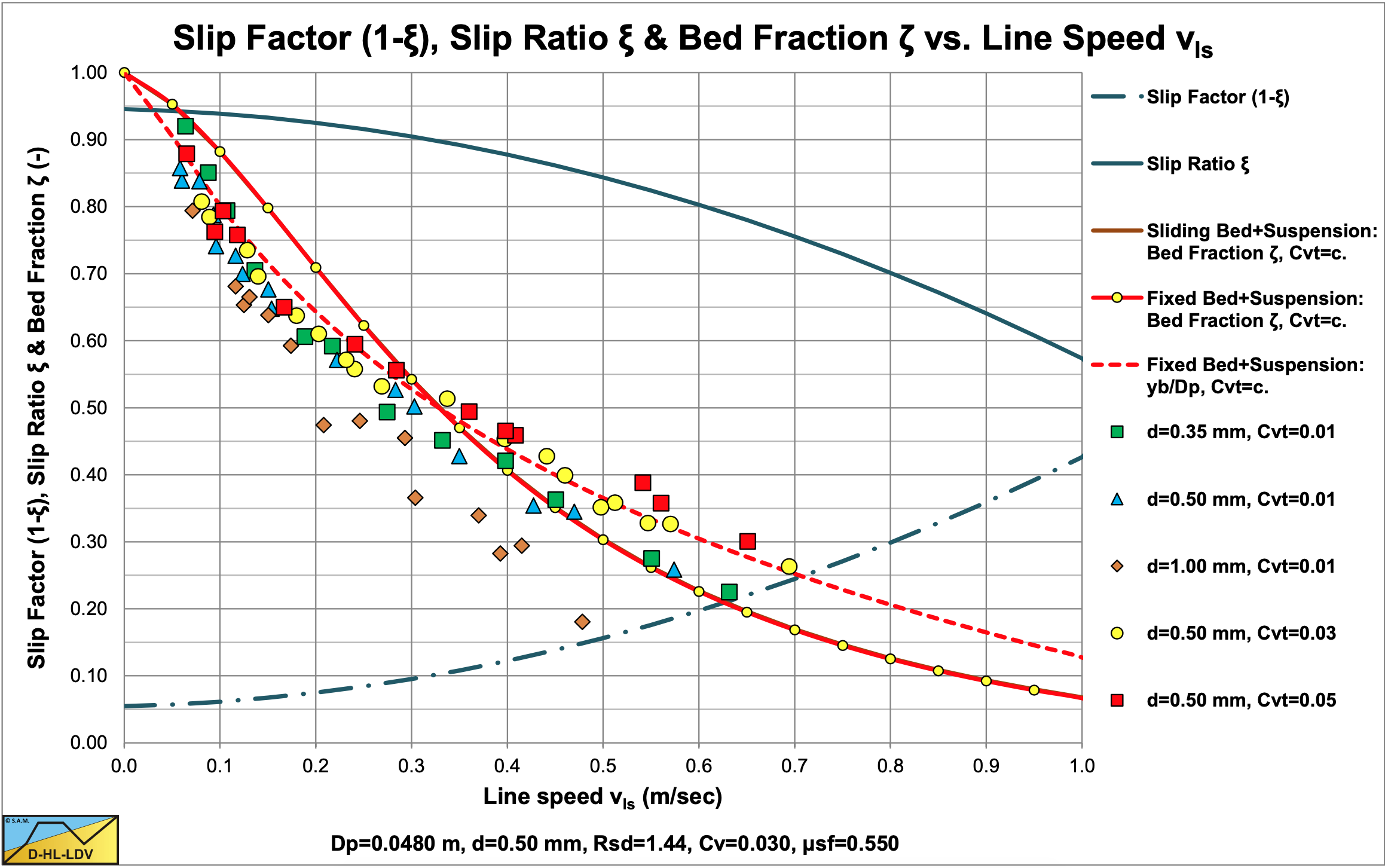
Doron & Barnea (1995) investigated the Limit of Stationary Deposit Velocity (LSDV), the Minimum Hydraulic Gradient Velocity (MHGV) and the bed height. The LSDV and MHGV, as shown in Figure 6.21-6, are from their own experiments. The 3 layer model overestimates the LSDV, while the DHLLDV Framework is closer to the experimental data. The 3 layer model is close to the MHGV, as is the DHLLDV Framework. Figure 6.21-7 shows bed height experiments of Harada et al. (1989) in a 120 mm x 30 mm conduit with particles with a density of 2.5 ton/m³. In terms of a hydraulic radius, this would match a circular pipe with a radius of 48 mm. The 3 layer model matches for 0.35 mm and 0.5 mm particles, but overestimates 1 mm particles. The figure shows the bed height according to the DHLLDV Framework, giving a good correlation for the 0.5 mm particle and a concentration of 0.03.

Resuming one can state that the Doron et al. (1987), Doron & Barnea (1993) and Doron & Barnea (1995) model and experiments contain some interesting concepts in addition to the Wilson (1979) 2 layer model. The use of concentration distributions based on open channel flow is however questionable. Not just for this research, but in general for all models discussed in this book.

Figure 6.21-6: The LSDV and MHGV according to Doron et al. (1987) and Doron & Barnea (1993).

Figure 6.21-7: Bed height measurements of Harada et al. (1989).

6.21.4 Some Issues

The additional force on top of the bed:

The use of the additional force, resulting from the Bagnold (1954) and (1957) stresses, on top of the bed by Doron et al. (1987), equation (6.21-7), is not so obvious. First of all an extra normal force on the bed requires enough submerged weight of particles on top of the bed, for example in a sheet flow or shear layer, where the shear forces are transferred by inter particle contacts. It is not explained where this force originates from. Secondly, if this force is transferred through the bed, resulting in additional normal stresses on the pipe wall, this force cannot be added to the normal force, but should be treated like the weight in the hydrostatic approach. According to the authors this force should not be present or at least there should be a check if the submerged weight of the particles above the bed justify this force, and thus will probably be compensated by the model later in order to match the experiments. For example by using a smaller sliding friction coefficient. The implementation of the Bagnold (1954) and (1957) stresses in the 3LM model is not correct, a stress balance does not exist, only a force balance. The Bagnold (1954) and (1957) stresses are implemented in a way that they appear on each surface.

This issue is present in both the 2LM and 3LM models.

The Darcy Weisbach friction factor at the interface:

The equation for the Darcy Weisbach friction factor at the interface, as used in the original article of Doron et al. (1987) seems a wrong interpretation of the Televantos et al. (1979) approach. The correct interpretation is given by equation (6.21-15).

The equation for the concentration at the bottom of the pipe:

It seems equation (6.21-28) in the original Doron et al. (1987) paper is incorrect (equation 33). There is no division by the integral. The correct equation is given here:

\[\ \mathrm{C_{vB}=\frac{\pi}{2}\cdot C_{vt}\cdot \frac{1}{\int_0^{\pi}e^{(-\frac{v_{th}}{\varepsilon}\cdot\frac{D_p}{2}\cdot(1-cos(\beta)))}\cdot sin^2(\beta)\cdot d\beta}} \]

Now for very small particles or very high velocities, the argument of the e-power gets close to zero, resulting in:

\[\ \mathrm{C_{v B}=\frac{\pi}{2} \cdot C_{v t} \cdot \frac{1}{\int_{0}^{\pi} \sin ^{2}(\beta) \cdot d \beta}=\frac{\pi}{2} \cdot C_{v t} \cdot \frac{1}{\frac{\pi}{2}}=C_{v t}}\]

The concentration at the bottom of the pipe equals the average concentration, also implying that the concentration is equal to the average concentration at any location in the pipe. A true homogeneous flow. With the original equation of Doron et al. (1987) this would give:

\[\ \mathrm{C}_{\mathrm{vB}}=\frac{\pi}{2} \cdot \mathrm{C}_{\mathrm{v t}} \cdot \int_{\mathrm{0}}^{\pi} \sin ^{2}(\beta) \cdot \mathrm{d} \beta=\frac{\pi}{2} \cdot \mathrm{C}_{\mathrm{v t}} \cdot \frac{\pi}{2}=\left(\frac{\pi}{2}\right)^{2} \cdot \mathrm{C}_{\mathrm{v t}} \approx \mathrm{2 . 5} \cdot \mathrm{C}_{\mathrm{v t}}\]

Which cannot be true for true homogeneous flow. The correct concentration distribution can be determined by substituting equation (6.21-45) in equation (6.21-26), giving:

\[\ \mathrm{C(y)=\frac{\pi}{2}\cdot C_{vt}\cdot \frac{e^{(-\frac{v_{th}}{\varepsilon}\cdot \frac{D_p}{2}\cdot (1-cos(\beta)))}}{\int_0^\pi e^{(-\frac{v_{th}}{\varepsilon}\cdot\frac{D_p}{2}\cdot (1-cos(\beta)))}\cdot sin^2(\beta)\cdot d\beta}} \]

Use of the concentration distribution to determine the LDV:

Doron et al. (1987) state that the critical velocity can be determined by evaluating the pressure gradient and finding the minimum pressure gradient line speed. This is referred to in this book as the Minimum Hydraulic Gradient Velocity (MHGV). What they did not conclude, a missed opportunity, is the velocity where the concentration at the bottom of the pipe equals the bed concentration. This is referred to in this book as the Limit Deposit Velocity. This occurs when, assuming the hindered terminal settling velocity is zero at bed concentration and the bed angle β is zero at the LDV:

\[\ \mathrm{ \int_{0}^{\pi} e^{\left(-\frac{v_{t h}}{\varepsilon} \cdot \frac{D_{p}}{2} \cdot(1-\cos (\beta))\right)} \cdot \sin ^{2}(\beta) \cdot d \beta=\frac{\pi}{2} \cdot \frac{C_{v t}}{C_{v b}}}\]

With the diffusion coefficient at the Limit Deposit Velocity:

\[\ \varepsilon=0.052 \cdot \mathrm{u}_{*} \cdot \mathrm{R} \quad\text{ with: }\quad \mathrm{u}_{*}=\sqrt{\frac{\lambda_{\mathrm{l}}}{\mathrm{8}}}{ \cdot \mathrm{v}_{\mathrm{l s}, \mathrm{l} \mathrm{d} \mathrm{v}}} \quad\text{ so: }\quad \varepsilon=\mathrm{0 . 0 5 2} \cdot \sqrt{\frac{\lambda_{\mathrm{l}}}{\mathrm{8}}}{ \cdot \mathrm{R} \cdot \mathrm{v}_{\mathrm{l} \mathrm{s}, \mathrm{l} \mathrm{d} \mathrm{v}}}\]

The relation for the Limit Deposit Velocity is defined:

\[\ \left.\int_{0}^{\pi} \mathrm{e}^{\left(-\frac{55}{\sqrt{\lambda_{\mathrm{l}}}} \cdot \frac{\mathrm{v}_{\mathrm{th}}}{\mathrm{v}_{\mathrm{s}, \mathrm{ldv}}} \cdot(1-\cos (\beta))\right.}\right) \cdot \sin ^{2}(\beta) \cdot \mathrm{d} \beta=\frac{\pi}{2} \cdot \frac{\mathrm{C}_{\mathrm{vt}}}{\mathrm{C}_{\mathrm{vb}}} \quad\text{ with: }\quad \lambda_{\mathrm{l}}=0.184 \cdot\left(\frac{\mathrm{v}_{\mathrm{ls}, \mathrm{ldv}} \cdot \mathrm{D}_{\mathrm{p}}}{v_{\mathrm{l}}}\right)^{-0.2}\]

This method however shows an LDV almost independent of the pipe diameter, continuously increasing with the terminal settling velocity (the particle diameter) and also results in very high LDV values, making it not suitable for the determination of the LDV and raising questions about the concentration distribution approach.

Use of the dynamic and static friction coefficients

In the 3LM model the dynamic friction coefficient is used for both the friction between the bed and the pipe wall and for the friction between the moving bed and the stationary bed. The latter is sand on sand friction and the internal friction angle should be used here. The sand on steel friction angle, or external friction angle is usually about 2/3 of the internal friction angle.

Figure 6.21-8: Data of Doron et al. (1987) and Doron & Barnea (1993) at very low concentrations.

Figure 6.21-9: Data of Doron et al. (1987) and Doron & Barnea (1993) at low concentrations, at the slifding flow criterion.

Figure 6.21-10: Data of Doron et al. (1987) and Doron & Barnea (1993) at low/medium concentrations.

Figure 6.21-11: Data of Doron et al. (1987) and Doron & Barnea (1993) at medium concentrations.

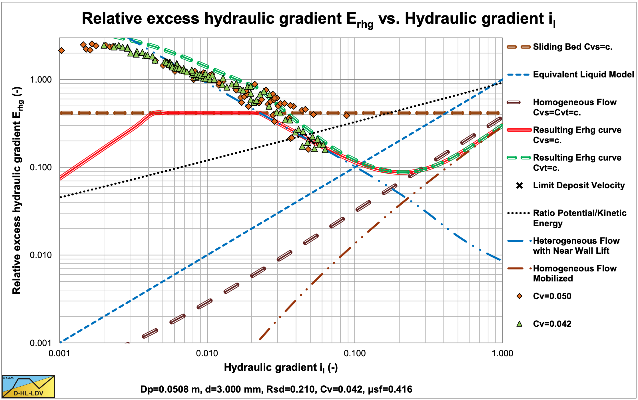
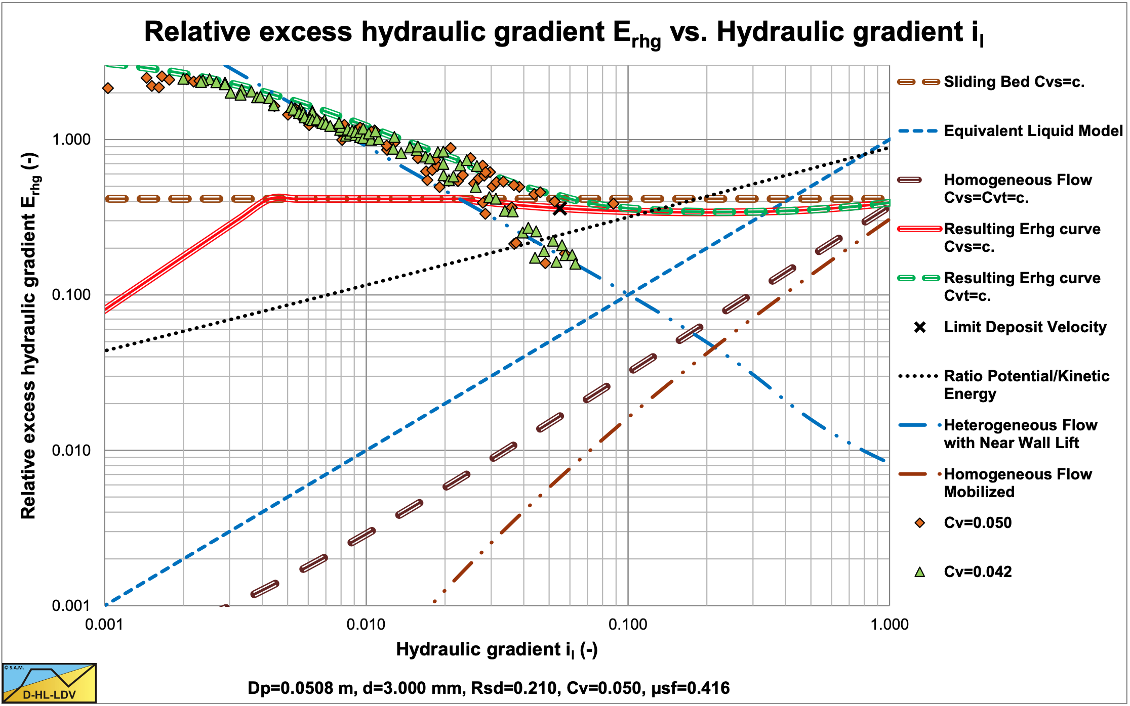
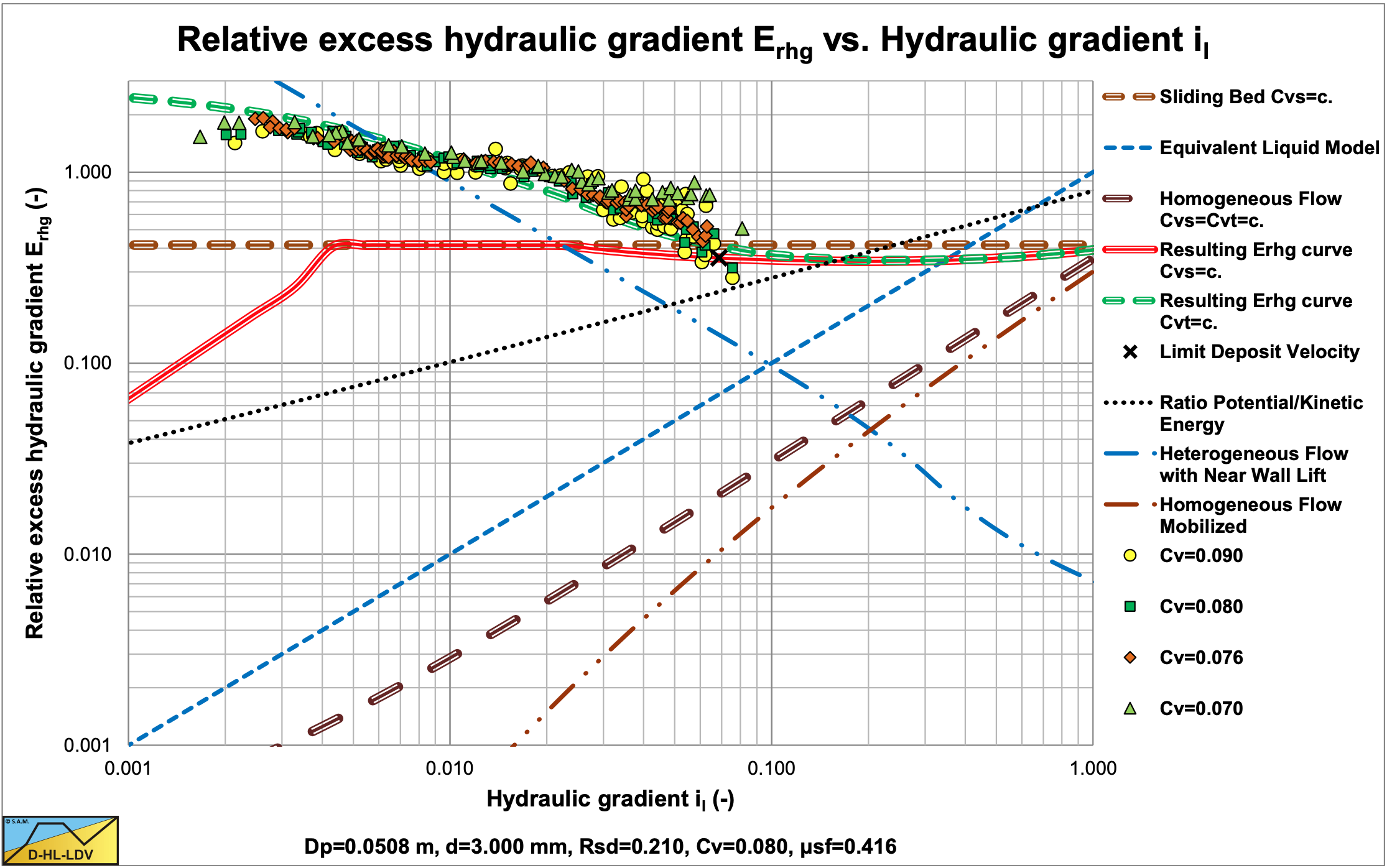
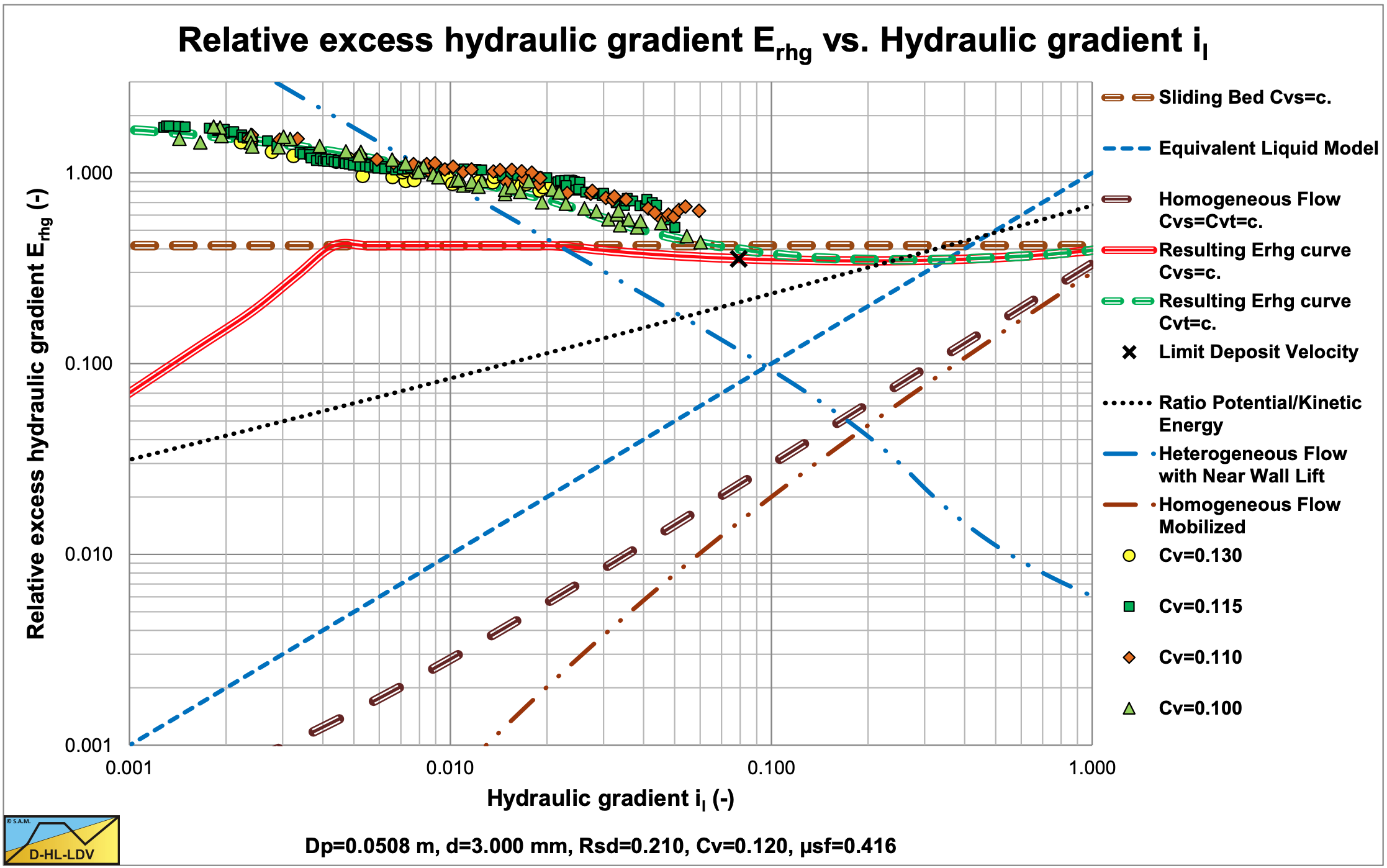
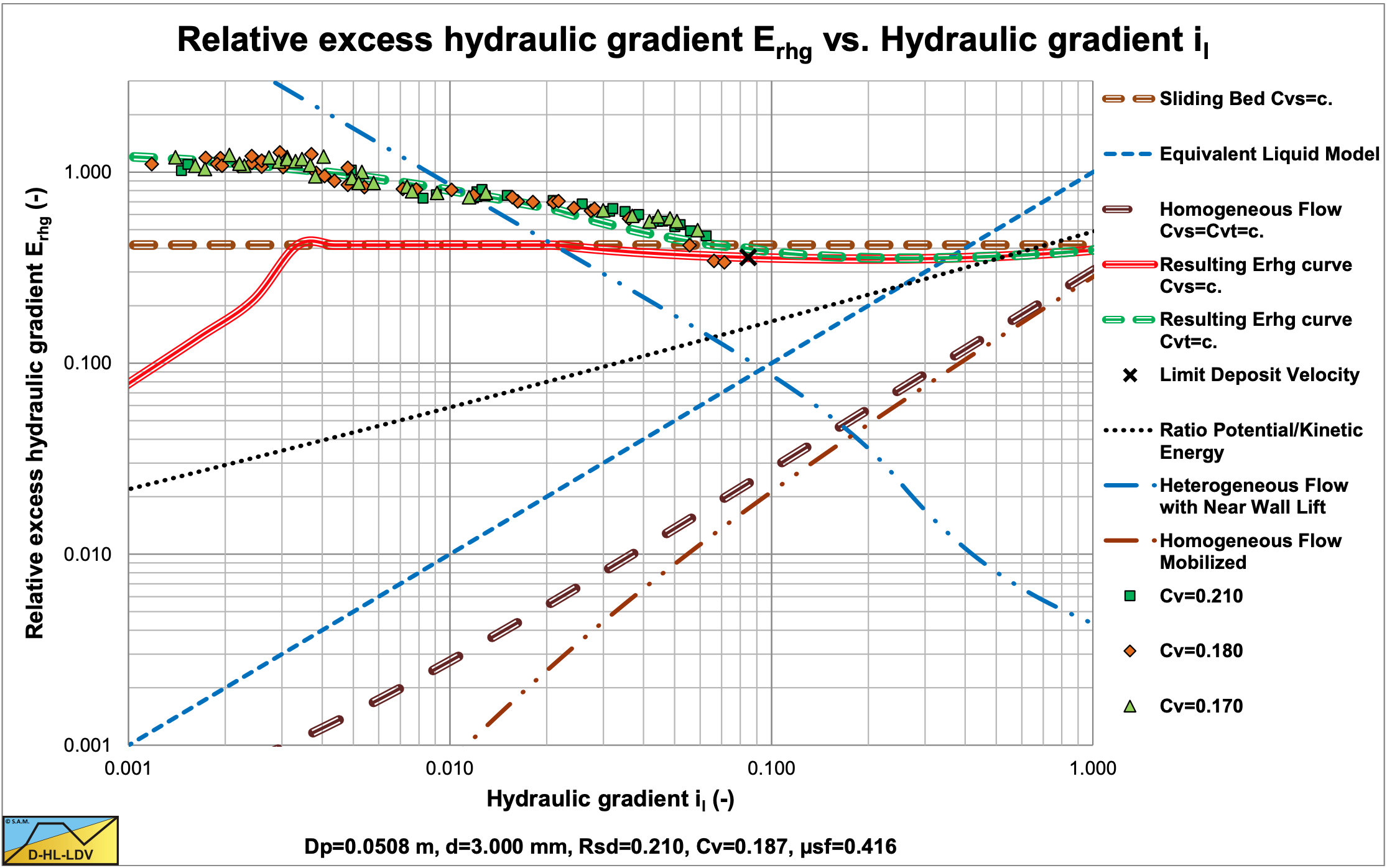
Figure 6.21-8 and Figure 6.21-9 show that for very low concentrations (C_vt<5%) the behavior at higher line speeds is according to the heterogeneous flow regime. At concentrations above 5% the behavior is according to the sliding flow regime. In this case the ratio of the particle diameter to the pipe diameter is 0.059, which is much larger than the ratio 0.015 as proposed by Wilson et al. (1992) as a criterion for full stratified flow.

Figure 6.21-12: Data of Doron et al. (1987) and Doron & Barnea (1993) at medium/high concentrations.

Figure 6.21-13: Data of Doron et al. (1987) and Doron & Barnea (1993) at high concentrations.

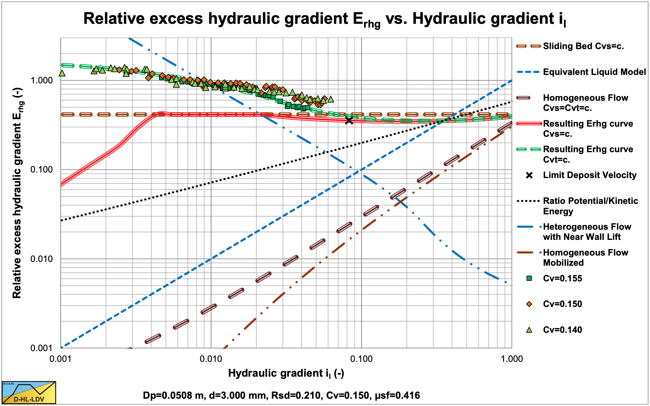
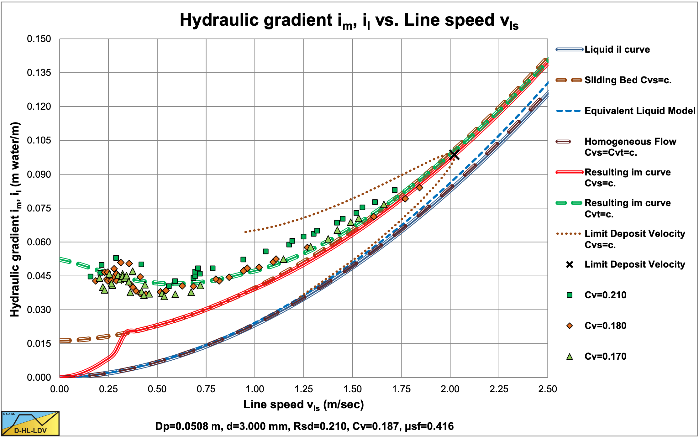
Figure 6.21-10, Figure 6.21-11 and Figure 6.21-12 show similar sliding flow behavior. The data of Doron et al. (1987) and Doron & Barnea (1993) are compared with the DHLLDV Framework and give a reasonable good match. Figure 6.21-13 and Figure 6.21-14 show the data as hydraulic gradient and relative excess hydraulic gradient. The comparison with the DHLLDV Framework is satisfactory.

It should be noted that all experiments were carried out below the LDV, so at relatively low line speeds. The concentrations measured were transport concentrations. This implies that at low line speeds there was either fixed bed or sliding bed transport and at the higher line speeds most probably sliding flow transport.

Figure 6.21-14: Data of Doron et al. (1987) and Doron & Barnea (1993) at high concentrations.

6.21.6 Modified Doron & Barnea Model

Based on the knowledge of today (2015) a number of modifications to the Doron & Barnea models are proposed. First of all, the Bagnold (1954) and (1957) stresses do not act on top of the moving bed, but can still be used to determine the thickness of the moving bed. Secondly the hydrostatic approach of Wilson (1979) to determine the normal force between the bed and the pipe wall is rejected, instead the weight approach of Miedema & Ramsdell (2014) is applied. The last main modification is using two different friction angles for internal friction and external friction. The force balances on the 3 layers do not change because of the modifications, but are given here for completeness of the model.

For the solids phase the continuity equation yields, neglecting slip between the two phases:

\[\ \mathrm{v}_{\mathrm{1}} \cdot \mathrm{A}_{\mathrm{1}} \cdot \mathrm{C}_{\mathrm{v s}, \mathrm{1}}+\mathrm{v}_{\mathrm{2}} \cdot \mathrm{A}_{\mathrm{2}} \cdot \mathrm{C}_{\mathrm{v b}}=\mathrm{v}_{\mathrm{l} \mathrm{s}} \cdot \mathrm{A}_{\mathrm{p}} \cdot \mathrm{C}_{\mathrm{v t}}\]

For the liquid phase the continuity equation yields, neglecting slip between the two phases:

\[\ \mathrm{v}_{1} \cdot \mathrm{A}_{1} \cdot\left(1-\mathrm{C}_{\mathrm{v s}, 1}\right)+\mathrm{v}_{2} \cdot \mathrm{A}_{2} \cdot\left(1-\mathrm{C}_{\mathrm{v b}}\right)=\mathrm{v}_{\mathrm{l} \mathrm{s}} \cdot \mathrm{A}_{\mathrm{p}} \cdot\left(1-\mathrm{C}_{\mathrm{v t}}\right)\]

The force balance on the heterogeneous layer yields, see Figure 6.21-2, similar to the 2LM model:

\[\ -\mathrm{A}_{1} \cdot \Delta \mathrm{p}=\mathrm{F}_{1, \mathrm{l}}+\mathrm{F}_{12, \mathrm{l}} \quad\text{ and }\quad-\mathrm{A}_{1} \cdot \frac{\Delta \mathrm{p}}{\Delta \mathrm{L}}=\tau_{1,\mathrm{l}} \cdot \mathrm{O}_{\mathrm{1}}+\tau_{12,1} \cdot \mathrm{O}_{12}\]

The force balance on the moving bed layer yields:

\[\ \begin{array}{left} -\mathrm{A}_{2} \cdot \Delta \mathrm{p}+\mathrm{F}_{12,\mathrm{l}}=\mathrm{F}_{20, \mathrm{sf}}+\mathrm{F}_{20,\mathrm{l}}+\mathrm{F}_{2, \mathrm{sf}}+\mathrm{F}_{2, \mathrm{\mathrm{l}}}\\
-\mathrm{A}_{2} \cdot \frac{\Delta \mathrm{p}}{\Delta \mathrm{L}}+\tau_{12,\mathrm{l}} \cdot \mathrm{O}_{12}=\tau_{20, \mathrm{sf}} \cdot \mathrm{O}_{20}+\tau_{20,\mathrm{l}} \cdot \mathrm{O}_{20}+\tau_{2, \mathrm{sf}} \cdot \mathrm{O}_{2}+\tau_{2,\mathrm{l}} \cdot \mathrm{O}_{2}\end{array}\]

Finally the force balance on the stationary bed layer yields:

\[\ -\mathrm{A}_{\mathrm{0}} \cdot \Delta \mathrm{p}+\mathrm{F}_{\mathrm{2 0}, \mathrm{s f}}+\mathrm{F}_{\mathrm{2 0}, \mathrm{l}}=\mathrm{F}_{\mathrm{0}, \mathrm{f}} \quad\text{ and }\quad-\mathrm{A}_{\mathrm{0}} \cdot \frac{\Delta \mathrm{p}}{\Delta \mathrm{L}}+\tau_{\mathrm{2 0}, \mathrm{s f}} \cdot \mathrm{O}_{\mathrm{2 0}}+\tau_{\mathrm{2 0}, \mathrm{l}} \cdot \mathrm{O}_{20}=\tau_{0, \mathrm{f}} \cdot \mathrm{O}_{\mathrm{0}}\]

The implementation of the forces resulting from liquid also have not changed (index l). The Darcy Weisbach shear stress \(\ \tau_{ 1,\mathrm{l}}\) is calculated with equation (6.21-11), similar to the 2LM model. The Darcy Weisbach shear stress \(\ \tau_{ 12,\mathrm{l}}\) is determined with equation (6.21-14), similar to the 2LM model. The Darcy Weisbach shear stress between the moving bed and the pipe wall \(\ \tau_{ 2,\mathrm{l}}\) is determined with equation (6.21-11), similar to the 2 LM model. The Darcy Weisbach shear stress between the moving bed and the stationary bed \(\ \tau_{ 20,\mathrm{l}}\) is calculated with equation (6.21-14), but of course with the velocities v₂ and v₀, similar to the 2LM model.

The implementation of the forces due to dynamic or static friction have changed (indices f and sf). In order to determine the friction forces, first the weight of each layer has to be determined.

The weight of the moving bed and the stationary bed F_W20 is:

\[\ \mathrm{F}_{\mathrm{W} \mathrm{2 0}}=\rho_{\mathrm{l}} \cdot \mathrm{g} \cdot \mathrm{\Delta L} \cdot \mathrm{R}_{\mathrm{s d}} \cdot \mathrm{C}_{\mathrm{v b}} \cdot \mathrm{A}_{\mathrm{p}} \cdot \frac{\left(\left(\beta_{\mathrm{0}}+\beta_{2}\right)-\sin \left(\beta_{0}+\beta_{2}\right) \cdot \cos \left(\beta_{0}+\beta_{2}\right)\right)}{\pi}\]

The weight of the stationary bed F_W0 is:

\[\ \mathrm{F}_{\mathrm{W} 0}=\rho_{\mathrm{l}} \cdot \mathrm{g} \cdot \Delta \mathrm{L} \cdot \mathrm{R}_{\mathrm{s} \mathrm{d}} \cdot \mathrm{C}_{\mathrm{v} \mathrm{b}} \cdot \mathrm{A}_{\mathrm{p}} \cdot \frac{\left(\left(\beta_{0}\right)-\sin \left(\beta_{0}\right) \cdot \cos \left(\beta_{0}\right)\right)}{\pi}\]

The weight of the moving bed F_W2 is:

\[\ \begin{array}{center} \mathrm{F}_{\mathrm{W} 2}=\mathrm{F}_{\mathrm{W} \mathrm{2 0}}-\mathrm{F}_{\mathrm{W} 0}=\rho_{\mathrm{l}} \cdot \mathrm{g} \cdot \Delta \mathrm{L} \cdot \mathrm{R}_{\mathrm{s} \mathrm{d}} \cdot \mathrm{C}_{\mathrm{v} \mathrm{b}} \cdot \mathrm{A}_{\mathrm{p}} \cdot \frac{\left(\left(\beta_{0}+\beta_{2}\right)-\sin \left(\beta_{0}+\beta_{2}\right) \cdot \cos \left(\beta_{0}+\beta_{2}\right)\right)}{\pi}\\
-\rho_{\mathrm{l}} \cdot \mathrm{g} \cdot \Delta \mathrm{L} \cdot \mathrm{R}_{\mathrm{s} \mathrm{d}} \cdot \mathrm{C}_{\mathrm{v} \mathrm{b}} \cdot \mathrm{A}_{\mathrm{p}} \cdot \frac{\left(\left(\beta_{0}\right)-\sin \left(\beta_{0}\right) \cdot \cos \left(\beta_{0}\right)\right)}{\pi}\end{array}\]

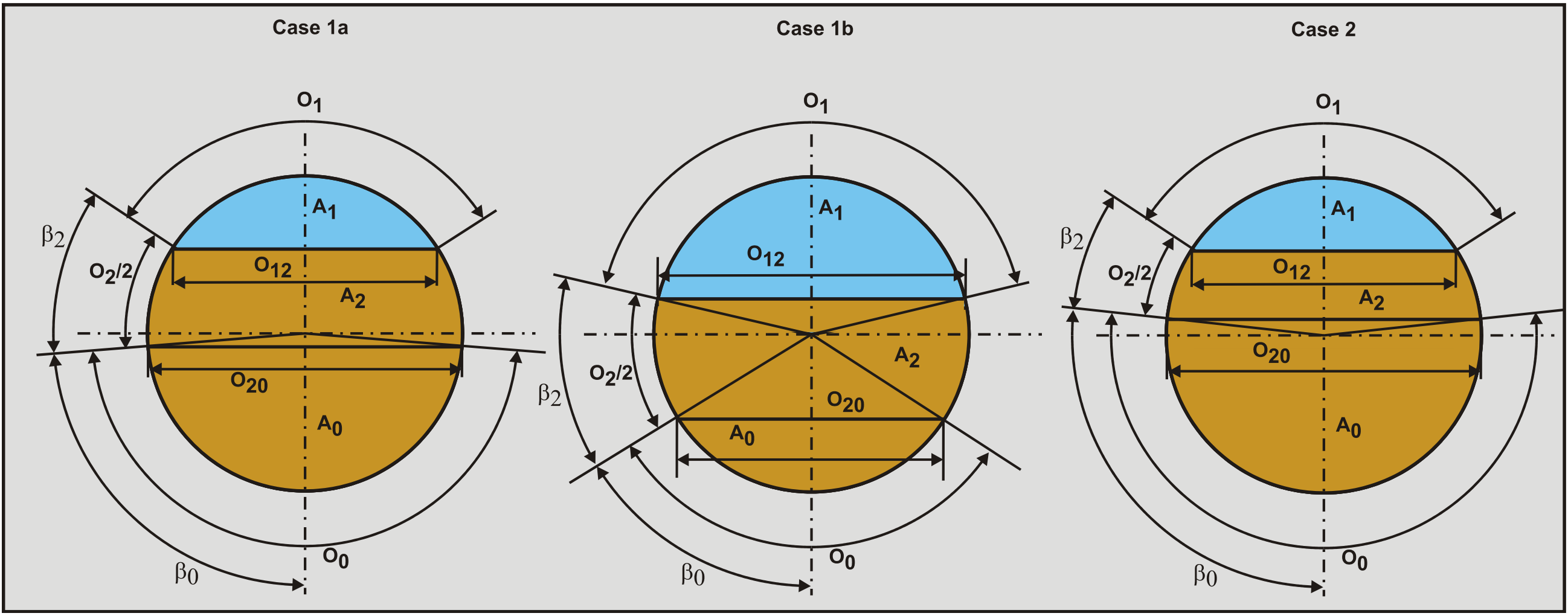
Now two cases have to be considered, the interface between the stationary and moving bed layers is below half the pipe diameter, or it is above half the pipe diameter. If it is below half the pipe diameter, part of the weight of the moving bed layer is carried by the pipe wall and the rest is carried by the interface. If it is above half the pipe diameter, the whole weight of the moving bed layer is carried by the interface. In the case it is below half the pipe diameter, again two cases have to be considered, the case where the width of the top of the moving bed layer is smaller than the interface width and the case where it is larger than the interface width. The 3 cases are discussed here:

Case 1a: The interface is below half the pipe diameter and the top width is smaller than the interface width.

Part of the weight of the moving bed layer is carried by the pipe wall. The rest is carried by the interface. The height of the moving bed layer is:

\[\ \begin{array}{left} \mathrm{y}_{\mathrm{b} 2} &=\left(\mathrm{y}_{\mathrm{b} 2}+\mathrm{y}_{\mathrm{b} 0}\right)-\mathrm{y}_{\mathrm{b} 0}=\frac{\mathrm{D}_{\mathrm{p}}}{\mathrm{2}} \cdot\left(\mathrm{1}-\cos \left(\boldsymbol{\beta}_{2}+\boldsymbol{\beta}_{\mathrm{0}}\right)\right)-\frac{\mathrm{D}_{\mathrm{p}}}{\mathrm{2}} \cdot\left(\mathrm{1}-\cos \left(\boldsymbol{\beta}_{\mathrm{0}}\right)\right) \\ &=\frac{\mathrm{D}_{\mathrm{p}}}{\mathrm{2}} \cdot\left(\cos \left(\beta_{\mathrm{0}}\right)-\cos \left(\boldsymbol{\beta}_{2}+\boldsymbol{\beta}_{\mathrm{0}}\right)\right) \end{array}\]

The part of the moving bed carried by the pipe wall F_W2,w is:

\[\ \left.{\mathrm{F}}_{\mathrm{W} 2, \mathrm{w}}=\rho_{\mathrm{l}} \cdot \mathrm{g} \cdot \Delta \mathrm{L} \cdot \mathrm{R}_{\mathrm{sd}} \cdot \mathrm{c}_{\mathrm{v} \mathrm{b}} \cdot \mathrm{2} \cdot\left(\begin{array}{l}\mathrm{A}_{\mathrm{p}} \cdot\left(\frac{\frac{\pi}{\mathrm{2}}-\left(\left(\beta_{0}\right)-\sin \left(\beta_{0}\right) \cdot \cos \left(\beta_{0}\right)\right)}{\pi}\right. \\ \mathrm{O}_{20} \cdot \frac{\mathrm{D}_{\mathrm{p}}}{2} \cdot\left(1-\cos \left(\beta_{0}\right)\right)\end{array}\right)\right)\]

The weight of the moving bed resting on the interface F_W2,i is now:

\[\ \mathrm{F}_{\mathrm{W} \mathrm{2}, \mathrm{i}}=\mathrm{F}_{\mathrm{W} 2}-\mathrm{F}_{\mathrm{W} \mathrm{2}, \mathrm{w}}\]

The force balance on the moving bed layer yields:

\[\ \begin{array}{left} -\mathrm{A}_{2} \cdot \Delta \mathrm{p}+\mathrm{F}_{12,\mathrm{l}}=\mathrm{F}_{20, \mathrm{s f}}+\mathrm{F}_{\mathrm{2} 0, \mathrm{l}}+\mathrm{F}_{2, \mathrm{s f}}+\mathrm{F}_{2, \mathrm{l}}\\
-\mathrm{A}_{2} \cdot \frac{\Delta \mathrm{p}}{\Delta \mathrm{L}}+\tau_{12,\mathrm{l}} \cdot \mathrm{O}_{12}=\tau_{20, \mathrm{s f}} \cdot \mathrm{O}_{20}+\tau_{20,\mathrm{l}} \cdot \mathrm{O}_{20}+\tau_{2, \mathrm{s f}} \cdot \mathrm{O}_{2}+\tau_{2,\mathrm{l}} \cdot \mathrm{O}_{2}\\
\mathrm{W i t h}: \\ \mathrm{F}_{20, \mathrm{s f}}=\mathrm{F}_{\mathrm{W} 2, \mathrm{i}} \cdot \tan (\varphi) \quad\text{ and }\quad \tau_{20, \mathrm{s} \mathrm{f}}=\frac{\mathrm{F}_{\mathrm{W} 2, \mathrm{i}} \cdot \tan (\varphi)}{\Delta \mathrm{L} \cdot \mathrm{O}_{20}}\\
\mathrm{F}_{2, \mathrm{s f}}=\mathrm{F}_{\mathrm{W} 2, \mathrm{w}} \cdot \tan \left(\frac{2}{3} \cdot \varphi\right) \quad\text{ and }\quad \tau_{2, \mathrm{sf}}=\frac{F_{\mathrm{W} 2, \mathrm{w}} \cdot \tan \left(\frac{2}{3} \cdot \varphi\right)}{\Delta \mathrm{L} \cdot \mathrm{O}_{20}}\end{array}\]

Finally the force balance on the stationary bed layer yields:

\[\ \begin{array}{left} &-\mathrm{A}_{0} \cdot \Delta \mathrm{p}+\mathrm{F}_{20, \mathrm{sf}}+\mathrm{F}_{20,\mathrm{l}}=\mathrm{F}_{0, \mathrm{f}} \quad\text{ and }\quad-\mathrm{A}_{\mathrm{0}} \cdot \frac{\Delta \mathrm{p}}{\Delta \mathrm{L}}+\tau_{20, \mathrm{sf}} \cdot \mathrm{O}_{20}+\tau_{20,\mathrm{l}} \cdot \mathrm{O}_{20}=\tau_{0, \mathrm{f}} \cdot \mathrm{O}_{0}\\
\text{With: }&\mathrm{F_{0, \mathrm{f}} \leq\left(F_{\mathrm{W} 2, \mathrm{i}}+F_{\mathrm{W} 0}\right) \cdot \tan \left(\frac{2}{3} \cdot \varphi\right)=\left(\mathrm{F}_{\mathrm{W} 2, \mathrm{i}}+\mathrm{F}_{\mathrm{W} 0}\right) \cdot \mu_{\mathrm{sf}}}\\
\text{and }&\tau_{0, \mathrm{f}} \leq \frac{\left(\mathrm{F}_{\mathrm{W} 2, \mathrm{i}}+\mathrm{F}_{\mathrm{W} 0}\right) \cdot \mu_{\mathrm{sf}}}{\Delta \mathrm{L} \cdot \mathrm{O}_{0}}\end{array}\]

Case 1b: The interface is below half the pipe diameter and the top width is larger than the interface width

The part of the weight carried by the interface is the weight of the cross section of the interface width times the thickness of the moving bed layer. The rest of the weight is carried by the pipe wall. The height of the moving bed layer is:

\[\ \begin{array}{left} \mathrm{y}_{\mathrm{b} 2} &=\left(\mathrm{y}_{\mathrm{b} 2}+\mathrm{y}_{\mathrm{b} 0}\right)-\mathrm{y}_{\mathrm{b} 0}=\frac{\mathrm{D}_{\mathrm{p}}}{\mathrm{2}} \cdot\left(\mathrm{1}-\cos \left(\boldsymbol{\beta}_{2}+\boldsymbol{\beta}_{\mathrm{0}}\right)\right)-\frac{\mathrm{D}_{\mathrm{p}}}{\mathrm{2}} \cdot\left(\mathrm{1}-\mathrm{c o s}\left(\boldsymbol{\beta}_{\mathrm{0}}\right)\right) \\ &=\frac{\mathrm{D}_{\mathrm{p}}}{\mathrm{2}} \cdot\left(\cos \left(\beta_{0}\right)-\cos \left(\beta_{2}+\beta_{0}\right)\right) \end{array}\]

The weight of the moving bed resting on the interface F_W2,i is:

\[\ \mathrm{F}_{\mathrm{W} \mathrm{2}, \mathrm{i}}=\rho_{\mathrm{l}} \cdot \mathrm{g} \cdot \Delta \mathrm{L} \cdot \mathrm{R}_{\mathrm{s} \mathrm{d}} \cdot \mathrm{C}_{\mathrm{v b}} \cdot \mathrm{y}_{\mathrm{b} \mathrm{2}} \cdot \mathrm{O}_{\mathrm{2} \mathrm{0}}\]

The weight of the moving bed resting on the pipe wall F_W2,w is now:

\[\ \mathrm{F}_{\mathrm{W} \mathrm{2}, \mathrm{w}}=\mathrm{F}_{\mathrm{W} \mathrm{2}}-\mathrm{F}_{\mathrm{W} \mathrm{2}, \mathrm{i}}\]

The force balance on the moving bed layer yields:

\[\ \begin{array}{left} &-\mathrm{A}_{2} \cdot \Delta \mathrm{p}+\mathrm{F}_{12,\mathrm{l}}=\mathrm{F}_{20, \mathrm{s f}}+\mathrm{F}_{\mathrm{2} 0, \mathrm{l}}+\mathrm{F}_{2, \mathrm{s f}}+\mathrm{F}_{2, \mathrm{l}}
\\
&-\mathrm{A}_{2} \cdot \frac{\Delta \mathrm{p}}{\Delta \mathrm{L}}+\tau_{12,\mathrm{l}} \cdot \mathrm{O}_{12}=\tau_{20, \mathrm{s f}} \cdot \mathrm{0}_{20}+\tau_{20,\mathrm{l}} \cdot \mathrm{O}_{20}+\tau_{2, \mathrm{s f}} \cdot \mathrm{O}_{2}+\tau_{2,\mathrm{l}} \cdot \mathrm{O}_{2}\\
\text{With: }& \mathrm{F}_{20, \mathrm{s f}}=\mathrm{F}_{\mathrm{W} 2, \mathrm{i}} \cdot \tan (\varphi) \quad\text{ and }\quad \tau_{20, \mathrm{s} \mathrm{f}}=\frac{\mathrm{F}_{\mathrm{W} 2, \mathrm{i}} \cdot \tan (\varphi)}{\Delta \mathrm{L} \cdot \mathrm{O}_{20}}\\
&\mathrm{F}_{2, \mathrm{s f}}=\mathrm{F}_{\mathrm{W} 2, \mathrm{w}} \cdot \tan \left(\frac{2}{3} \cdot \varphi\right) \quad\text{ and }\quad \tau_{2, \mathrm{sf}}=\frac{F_{\mathrm{W} 2, \mathrm{w}} \cdot \tan \left(\frac{2}{3} \cdot \varphi\right)}{\Delta \mathrm{L} \cdot \mathrm{O}_{20}}\end{array}\]

Finally the force balance on the stationary bed layer yields:

\[\ \begin{array}{left}&-\mathrm{A}_{0} \cdot \Delta \mathrm{p}+\mathrm{F}_{20, \mathrm{sf}}+\mathrm{F}_{20,\mathrm{l}}=\mathrm{F}_{0, \mathrm{f}} \quad\
text{ and }\quad-\mathrm{A}_{0} \cdot \frac{\Delta \mathrm{p}}{\Delta \mathrm{L}}+\tau_{20, \mathrm{sf}} \cdot \mathrm{O}_{20}+\tau_{20,\mathrm{l}} \cdot \mathrm{O}_{20}=\tau_{0, \mathrm{f}} \cdot \mathrm{O}_{0}\\
\text{With: }& F_{0, \mathrm{f}} \leq\left(F_{\mathrm{W} 2, \mathrm{i}}+F_{\mathrm{W} 0}\right) \cdot \tan \left(\frac{2}{3} \cdot \varphi\right)=\left(\mathrm{F}_{\mathrm{W} 2, \mathrm{i}}+\mathrm{F}_{\mathrm{W} 0}\right) \cdot \mu_{\mathrm{sf}}\\
\text{and }&\tau_{0, \mathrm{f}} \leq \frac{\left(\mathrm{F}_{\mathrm{W} 2, \mathrm{i}}+\mathrm{F}_{\mathrm{W} 0}\right) \cdot \mu_{\mathrm{sf}}}{\Delta \mathrm{L} \cdot \mathrm{O}_{0}}\end{array}\]

Case 2: The interface is above half the pipe diameter and the top width is always smaller than the interface width

The full weight of the moving bed layer is resting on the interface. The resisting shear force on the interface due to internal friction F_20,sf + the viscous friction force F_20,l have to be equal to the shear force on top of the moving bed F_12,l + the pressure force –A₂·Δp.

The force balance on the moving bed layer reduces to:

\[\ \begin{array}{left} -\mathrm{A}_{2} \cdot \Delta \mathrm{p}+\mathrm{F}_{12, \mathrm{l}}=\mathrm{F}_{\mathrm{2} 0, \mathrm{s f}}+\mathrm{F}_{\mathrm{2} 0, \mathrm{l}} \quad\text{ and }\quad-\mathrm{A}_{2} \cdot \frac{\Delta \mathrm{p}}{\Delta \mathrm{L}}+\tau_{12,\mathrm{l}} \cdot \mathrm{O}_{12}=\tau_{20, \mathrm{sf}} \cdot \mathrm{O}_{20}+\tau_{20,\mathrm{l}} \cdot \mathrm{O}_{20}\\
\text{With } \quad \mathrm{F}_{20, \mathrm{s f}}=\mathrm{F}_{\mathrm{W} 2} \cdot \tan (\varphi) \quad\text{ and }\quad \tau_{20, \mathrm{s f}}=\frac{\mathrm{F}_{\mathrm{W} 2} \cdot \tan (\varphi)}{\Delta \mathrm{L} \cdot \mathrm{O}_{20}}\end{array}\]

Finally the force balance on the stationary bed layer yields:

\[\ \begin{array}{left}-\mathrm{A}_{0} \cdot \Delta \mathrm{p}+\mathrm{F}_{20, \mathrm{s f}}+\mathrm{F}_{20,\mathrm{l}}=\mathrm{F}_{\mathrm{0}, \mathrm{f}} \quad
\text{ and }\quad-\mathrm{A}_{\mathrm{0}} \cdot \frac{\Delta \mathrm{p}}{\Delta \mathrm{L}}+\tau_{20, \mathrm{s f}} \cdot \mathrm{O}_{20}+\tau_{20,\mathrm{l}} \cdot \mathrm{O}_{20}=\tau_{0, \mathrm{f}} \cdot \mathrm{O}_{\mathrm{0}}\\
\text{With: }\quad \mathrm{F}_{\mathrm{0}, \mathrm{f}} \leq \mathrm{F}_{\mathrm{W} \mathrm{2 0}} \cdot \tan \left(\frac{2}{\mathrm{3}} \cdot \varphi\right)=\mathrm{F}_{\mathrm{W} \mathrm{2 0}} \cdot \mu_{\mathrm{s f}} \quad\text{ and }\quad \tau_{0, \mathrm{f}}=\frac{\mathrm{F}_{\mathrm{W} 20} \cdot \mu_{\mathrm{sf}}}{\Delta \mathrm{L} \cdot \mathrm{O}_{\mathrm{0}}}\end{array}\]

Solution Procedure:

First assume all the solids are in a stationary bed. This results in β₀+β₂ based on the volumetric concentration given. Based on this total bed angle the velocity above the bed can be determined. Once the velocity is known the concentration distribution above the bed can be determined and the heterogeneous fraction and bed fraction are known. Now the bed height has to be adjusted in order to satisfy the continuity equations.

The Darcy Weisbach friction factors on the pipe wall and the bed interface can be determined, resulting in the pressure gradient in the heterogeneous layer. Once the pressure gradient is known, the force balance on the moving bed layer can be determined assuming a certain β₂. By iteration a force balance on the moving bed layer should be achieved, resulting in a matching β₂ and moving bed velocity v₂.

Now that the forces are known on the stationary bed and the bed angle β₀ is known, the force balance on the stationary bed can be determined. If the resulting friction force between the stationary bed and the pipe wall is smaller than the maximum, the stationary bed is really stationary, but if it’s larger, the whole bed is moving/sliding. In the case of a true stationary bed, the Darcy Weisbach friction coefficients have to be adjusted for the moving bed velocity and the procedure has to be repeated.

In the case of a sliding bed (the whole bed is sliding) the 2LM model has to be applied. This can be achieved by taking β₀=0.

Figure 6.21-15: The 3 cases.

6.21.7 Inclined Pipes

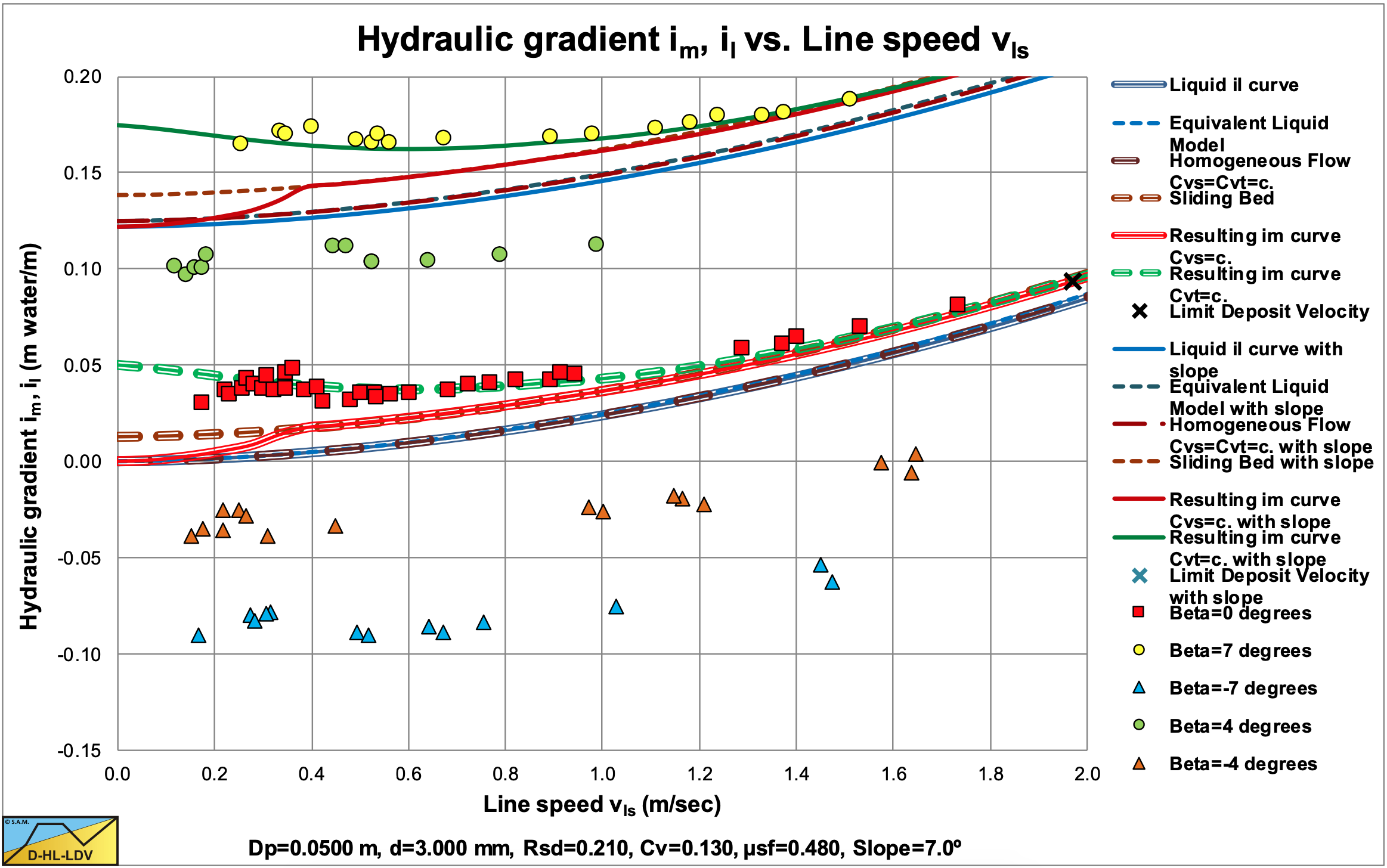
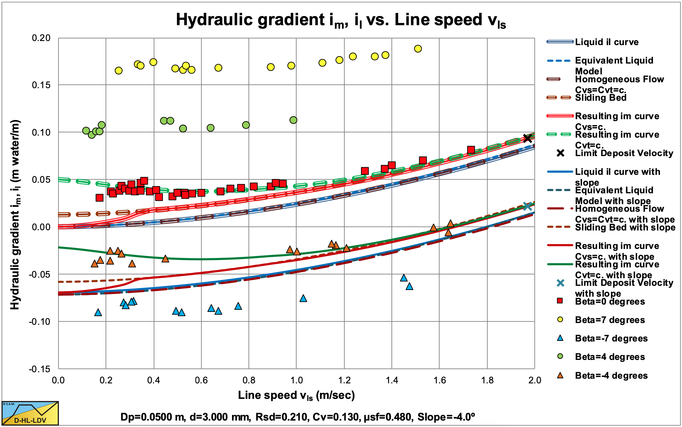
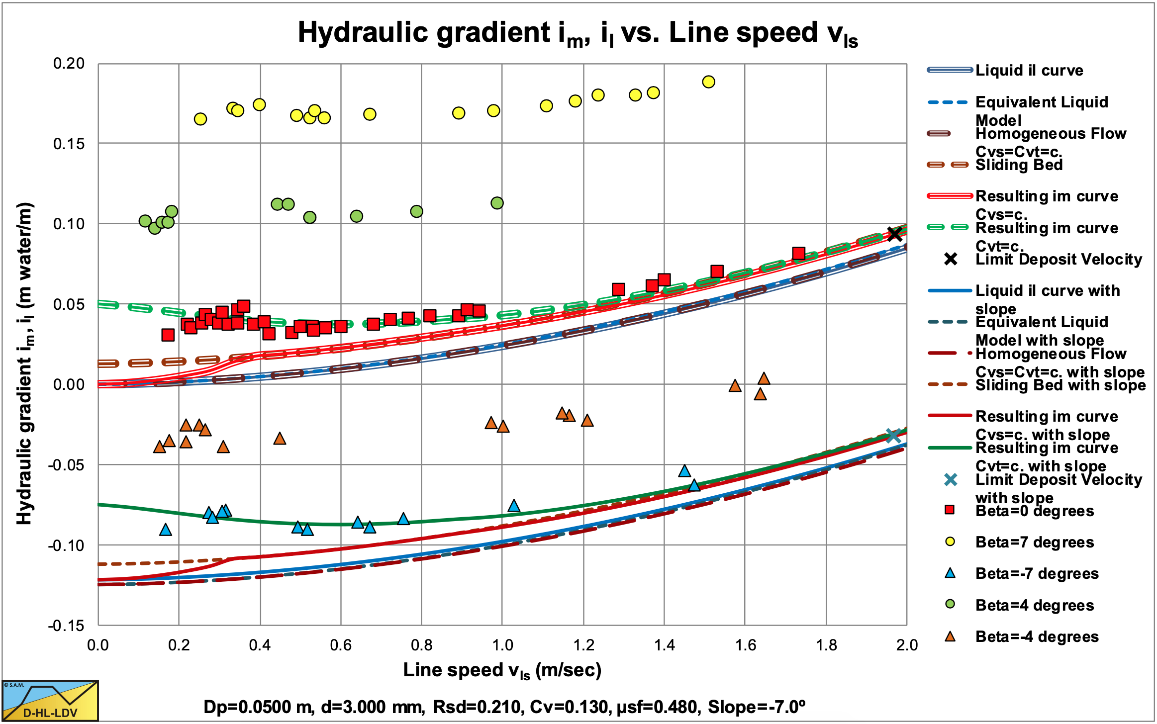
Doron et al. (1997) investigated the influence of inclined pipes, based on their 2LM and 3LM models. Basically they multiplied the sliding friction with the cosine of the inclination angle and they added the potential energy term, which is proportional with the sine of the inclination angle. They carried out experiments with inclination angles from -7 to +7 degrees. The resulting data however is dominated by the potential energy term.

They also investigated the Limit of Stationary Deposit Velocity (LSDV), the start of a sliding bed. Ascending pipes show an increasing LSDV with a maximum for an inclination angle of about 15 degrees, while descending pipes show a sharp decrease of the LSDV, because gravity becomes the driving force. At a certain negative inclination angle the bed will start sliding downwards because of gravity. It should be mentioned that Doron et al. (1997) use the delivered volumetric concentration, while LSDV models are usually based on spatial volumetric concentration. Especially in the stationary and sliding bed regimes the difference is significant.

Figure 6.21-16: The data of Doron et al. (1997) versus
the DHLLDV Framework for a horizontal and a 7^o ascending pipe.

Figure 6.21-17: The data of Doron et al. (1997) versus
the DHLLDV Framework for a horizontal and a 4^o ascending pipe.

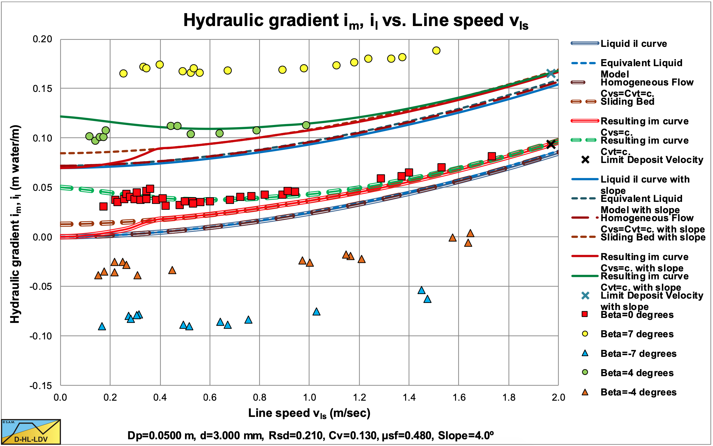
Figure 6.21-16, Figure 6.21-17, Figure 6.21-18 and Figure 6.21-19 show the data of Doron et al. (1997) versus the DHLLDV Framework for a horizontal pipe and a 4^o and 7^o ascending pipe and a 4^o and 7^o descending pipe. The solid green lines show the hydraulic gradient for the delivered volumetric concentration. In general the theoretical curves and the experimental data match well, although at very low line speeds the experimental points are lower than the theoretical curves. The theoretical curves are based on a sliding bed and it is possible that at very low line speeds there is a stationary bed, resulting in smaller hydraulic gradients, since the sliding friction is not fully mobilized. The difference between a horizontal pipe and the inclined pipes is dominated by the potential energy term (the sine), since the cosine is larger than 0.99 for the inclination angles considered, while the sine has a value of 0.12 for a 7^o inclination angle. Much larger inclination angles are required to see the influence of the cosine on the sliding friction.

Figure 6.21-18: The data of Doron et al. (1997) versus
the DHLLDV Framework for a horizontal and a 4^o descending pipe.

Figure 6.21-19: The data of Doron et al. (1997) versus
the DHLLDV Framework for a horizontal and a 7^o descending pipe.

6.21.8 Nomenclature Doron & Barnea Models

Ap	Cross section pipe	m^2
A0	Cross section stationary bed	m^2
A1	Cross section above bed, heterogeneous flow	m^2
A2	Cross section moving/sliding bed	m^2
C	Spatial volumetric concentration	-
Cvb	Volumetric spatial bed concentration	-
CvB	Volumetric spatial bottom concentration	-
Cvs	Spatial volumetric concentration	-
Cvs,0	Spatial volumetric concentration in cross section 0	-
Cvs,1	Spatial volumetric concentration in cross section 1	-
Cvs,2	Spatial volumetric concentration in cross section 2	-
Cvt	Delivered (transport) volumetric concentration	-
d	Particle diameter	m
DH1	Hydraulic diameter cross section 1, heterogeneous flow	m
DH2 ​​​​​​​	Hydraulic diameter cross section 2, moving/sliding bed	m
Dp	Pipe diameter	m
Erhg	Relative excess hydraulic gradient	-
F0,f	Static friction force between stationary bed and pipe wall	kN
F1,l	Force between liquid and pipe wall	kN
F12,l	Force between liquid and moving/sliding bed	kN
F2,sf	Force on bed due to friction with the pipe wall	kN
F2,l	Force on bed due to pore liquid	kN
F20,sf	Force due to friction between moving and stationary bed	kN
F20,l	Force on moving bed due to viscous losses at the interface moving – stationary bed	kN
FN	Normal force	kN
FN0 ​​​​​​​	Normal force stationary bed – pipe wall	kN
FN1 ​​​​​​​	Normal force based on the weight of the bed	kN
FN2 ​​​​​​​	Normal force based on the shear stress on the bed	kN
FN2	Normal force moving bed - pipe wall	kN
FN20	Normal force moving bed - stationary bed	kN
FW0	Weight stationary bed	kN
FW2	Weight moving bed	kN
FW2,i	Weight moving bed on interface	kN
FW2,w	Weight moving bed on pipe wall	kN
FW20	Weight moving bed + stationary bed	kN
g	Gravitational constant 9.81 m/s^2	m/s^2
il	Hydraulic gradient liquid	-
ΔL	Length of pipe section	m
LDV	Limit Deposit Velocity	m/s
LSDV	Limit of Stationary Deposit Velocity	m/s
Op	Circumference pipe	m
O0 ​​​​​​​	Circumference pipe stationary bed	m
O1 ​​​​​​​	Circumference pipe above bed, heterogeneous flow	m
O2 ​​​​​​​	Circumference pipe moving/sliding bed	m
O12	Width of top of bed	m
O20	Width interface moving bed – stationary bed	m
Δp	Pressure difference	kPa
Δp1 ​​​​​​​	Pressure difference on cross section 1	kPa
Δp2 ​​​​​​​	Pressure difference on cross section 2	kPa
Re	Reynolds number	-
Rsd	Relative submerged density	-
R	Pipe radius	m
u*	Friction velocity	m/s
vt	Terminal settling velocity	m/s
vth	Terminal settling velocity hindered	m/s
vls	Line speed	m/s
v0 ​​​​​​​	Cross section averaged velocity stationary bed v0=0	m/s
v1 ​​​​​​​	Cross section averaged velocity above bed, heterogeneous region	m/s
v2 ​​​​​​​	Cross section averaged velocity moving/sliding bed	m/s
y	Vertical coordinate in pipe	m
yb	Height of bed	m
yb0	Height of stationary bed	m
yb2	Height of moving/sliding bed	m
α1 ​​​​​​​	Proportionality factor Darcy Weisbach friction factor cross section 1	-
α2 ​​​​​​​	Proportionality factor Darcy Weisbach friction factor cross section 2	-
β	Bed angle	rad
β0	Bed angle stationary bed	rad
β2	Bed angle moving/sliding bed	rad
β	Richardson & Zaki hindered settling power	-
β1 ​​​​​​​	Power Darcy Weisbach friction factor cross section 1	-
β2 ​​​​​​​	Power Darcy Weisbach friction factor cross section 2	-
ε	Pipe wall roughness	m
ε	Diffusivity	m/s
ρl	Density carrier liquid	ton/m^3
ρs	Density solids	ton/m^3
ρ1 ​​​​​​​	Density of fluid in cross section 1	ton/m^3
ρ2 ​​​​​​​	Density of fluid in cross section 2	ton/m^3
φ	Angle of internal friction bed	o
λ1 ​​​​​​​	Darcy-Weisbach friction factor with pipe wall	-
λ2 ​​​​​​​	Darcy-Weisbach friction factor with pipe wall, liquid in bed	-
λ12	Darcy-Weisbach friction factor on the bed	-
\(\ v_{\mathrm{l}} \)	Kinematic viscosity	m^2/s
\(\ \tau_{ 0, \mathrm{f}, \mathrm{max}}\)	Maximum shear stress stationary bed – pipe wall	kPa
\(\ \tau_{1,\mathrm{l}}\)	Shear stress liquid-pipe wall above bed	kPa
\(\ \tau_{ 12,\mathrm{l}}\)	Shear stress bed-liquid interface	kPa
\(\ \tau_{2,\mathrm{l}}\)	Shear stress liquid-pipe in bed, sliding bed – pipe wall	kPa
\(\ \tau_{ 2, \mathrm{sf}}\)	Shear stress from sliding friction, sliding bed – pipe wall	kPa
\(\ \tau_{ 20,\mathrm{sf}}\)	Shear stress moving bed – stationary bed	kPa
μsf	Sliding friction coefficient	-
μl	Dynamic viscosity liquid	Pa·s