7.8: The Limit Deposit Velocity

7.8.1 Introduction

When the flow velocity decreases, there will be a moment where sedimentation of the particles starts to occur. The corresponding line speed is called the Limit Deposit Velocity. Often other terms are used like the critical velocity, critical deposition velocity, deposit velocity, deposition velocity, settling velocity, minimum velocity or suspending velocity. Here we will use the term Limit Deposit Velocity. This Limit Deposit Velocity may be considered the transition between two different flow regimes, however for most sands it will be somewhere in the heterogeneous regime. The possible transitions are shown in Table 7.8-1. The transitions fixed bed to sliding bed (Limit of Stationary Deposit Velocity) is not considered to be the Limit Deposit Velocity, because it is followed by the transition sliding bed or fixed bed to heterogeneous transport, which is considered to be one of the 3 possible Limit Deposit Velocities. The other 2 are; the LDV close to the transition of heterogeneous transport to homogeneous transport and the LDV somewhere in the heterogeneous regime. The Limit of Sliding Bed Velocity (LSBV), the transition of the sliding bed regime with the homogeneous regime, is always at very high line speeds beyond the operational range.

Table 7.8-1: Possible transitions.

	Fixed Bed	Sliding Bed	Heterogeneous	Homogeneous (ELM)
Fixed Bed		LSDV	LDV (Fine & Medium)
Sliding Bed			LDV (Coarse)	LSBV
Heterogeneous				LDV (Very Fine)
Homogeneous

The 5 transition velocities can be determined knowing the equations for the hydraulic gradient in the different regimes. These equations are:

The homogeneous regime, according to the ELM:

\[\ \mathrm{i}_{\mathrm{m}}=\mathrm{i}_{\mathrm{l}} \cdot\left(\mathrm{1}+\mathrm{R}_{\mathrm{s d}} \cdot \mathrm{C}_{\mathrm{v s}}\right)\]

And for the relative excess hydraulic gradient:

\[\ \mathrm{E}_{\mathrm{r h g}}=\frac{\mathrm{i}_{\mathrm{m}}-\mathrm{i}_{\mathrm{l}}}{\mathrm{R}_{\mathrm{s d}} \cdot \mathrm{C}_{\mathrm{v s}}}=\mathrm{i}_{\mathrm{l}}\]

The heterogeneous regime:

\[\ \mathrm{i}_{\mathrm{m}}=\mathrm{i}_{\mathrm{l}} \cdot\left(1+\frac{\left(2 \cdot \mathrm{g} \cdot \mathrm{R}_{\mathrm{s} \mathrm{d}} \cdot \mathrm{D}_{\mathrm{p}}\right)}{\lambda_{\mathrm{l}}} \cdot \mathrm{C}_{\mathrm{v} \mathrm{s}} \cdot \frac{\mathrm{1}}{\mathrm{v}_{\mathrm{ls}}^{2}} \cdot\left(\frac{\mathrm{v}_{\mathrm{t}}}{\mathrm{v}_{\mathrm{ls}}} \cdot\left(1-\frac{\mathrm{C}_{\mathrm{v} \mathrm{s}}}{\mathrm{\kappa}_{\mathrm{C}}}\right)^{\beta}+\frac{\mathrm{8 . 5}^{2}}{\lambda_{\mathrm{l}}} \cdot\left(\frac{\mathrm{v}_{\mathrm{t}}}{\sqrt{\mathrm{g} \cdot \mathrm{d}}}\right)^{\mathrm{1 0 / 3}} \cdot\left(\frac{\left(v_{\mathrm{l}} \cdot \mathrm{g}\right)^{1 / 3}}{\mathrm{v}_{\mathrm{l s}}}\right)^{2}\right)\right)\]

And for the relative excess hydraulic gradient:

\[\ \mathrm{E}_{\mathrm{r h g}}=\frac{\mathrm{i}_{\mathrm{m}}-\mathrm{i}_{\mathrm{l}}}{\mathrm{R}_{\mathrm{s d}} \cdot \mathrm{C}_{\mathrm{v s}}}=\frac{\mathrm{v}_{\mathrm{t}}}{\mathrm{v}_{\mathrm{l s}}} \cdot\left(\mathrm{1}-\frac{\mathrm{C}_{\mathrm{v s}}}{\mathrm{\kappa}_{\mathrm{C}}}\right)^{\beta}+\frac{\mathrm{8 .5}^{2}}{\lambda_{\mathrm{l}}} \cdot\left(\frac{\mathrm{v}_{\mathrm{t}}}{\sqrt{\mathrm{g} \cdot \mathrm{d}}}\right)^{\mathrm{10} / \mathrm{3}} \cdot\left(\frac{\left(v_{\mathrm{l}} \cdot \mathrm{g}\right)^{1 / 3}}{\mathrm{v}_{\mathrm{ls}}}\right)^{2}\]

The sliding bed regime:

\[\ \mathrm{i}_{\mathrm{m}}=\mathrm{i}_{\mathrm{l}} \cdot\left(\mathrm{1}+\mu_{\mathrm{s f}} \cdot \frac{\left(\mathrm{2} \cdot \mathrm{g} \cdot \mathrm{R}_{\mathrm{s d}} \cdot \mathrm{D}_{\mathrm{p}}\right)}{\lambda_{\mathrm{l}}} \cdot \mathrm{C}_{\mathrm{v s}} \cdot \frac{\mathrm{1}}{\mathrm{v}_{\mathrm{l s}}^{2}}\right)\]

And for the relative excess hydraulic gradient:

\[\ \mathrm{E}_{\mathrm{r h g}}=\frac{\mathrm{i}_{\mathrm{m}}-\mathrm{i}_{\mathrm{l}}}{\mathrm{R}_{\mathrm{s d}} \cdot \mathrm{C}_{\mathrm{v s}}}=\mu_{\mathrm{sf}}\]

For the LDV in the heterogeneous regime a different approach has to be applied. This statement is based on the analysis of many public available data. The transition velocities found, always lie in between the transition velocity of a sliding bed to heterogeneous transport and the transition velocity of heterogeneous to homogeneous transport. This will be discussed in a next paragraph.

The Limit Deposit Velocity is defined here as the line speed above which there is no stationary bed or sliding bed, Thomas (1962). Below the LDV there may be either a stationary or fixed bed or a sliding bed. For the critical velocity often the Minimum Hydraulic Gradient Velocity (MHGV) is used, Wilson (1942). For higher concentrations this MHGV may be close to the LDV, but for lower concentrations this is certainly not the case. Yagi et al. (1972) reported using the MHGV, making the data points for the lower concentrations to low, which is clear from Figure 7.8-1.

Another weak point of the MHGV is, that it depends strongly on the model used for the heterogeneous flow regime. Durand and Condolios (1952), Fuhrboter (1961), Jufin and Lopatin (1966) and others will each give a different MHGV. In dredging the process is instationary, meaning a constantly changing PSD and concentration in long pipelines, making it almost impossible to determine the MHGV.

Wilson (1979) derived a method for determining the transition velocity between the stationary bed and the sliding bed, which is named here the Limit of Stationary Deposit Velocity (LSDV). Since the transition stationary bed versus sliding bed, the LSDV, will always give a smaller velocity value than the moment of full suspension or saltation, the LDV, one should use the LDV, to be sure there is no deposit at all. For small particles it is also possible that the bed is already completely suspended before the bed could ever start sliding (theoretically). In that case an LSDV does not even exist. This is the reason for choosing the LDV as the critical velocity and developing a new model for this, independent of the head loss model and always existing.

The Froude number F_L is often used for the LDV, because it allows comparison of the LDV for different pipe diameters D_p and relative submerged densities R_sd without having to change the scale of the graph, this is defined as:

\[\ \mathrm{F}_{\mathrm{L}}=\frac{\mathrm{v}_{\mathrm{l} \mathrm{s}, \mathrm{l} \mathrm{d} \mathrm{v}}}{\sqrt{\mathrm{2 \cdot \mathrm { g } \cdot \mathrm { R } _ { \mathrm { s d } } \cdot \mathrm { D } _ { \mathrm { p } }}}}=\frac{\mathrm{L} \mathrm{D} \mathrm{V}}{\sqrt{\mathrm{2 \cdot g \cdot R}_{\mathrm{s d}} \cdot \mathrm{D}_{\mathrm{p}}}}\]

The research consisted of two parts, analyzing the experimental data and analyzing the resulting models based on these data. First the experimental data will be discussed. It should be noted that sometimes the 2 and the relative submerged density R_sd are omitted. Because there are numerous data and equations for the critical velocity (LSDV, LDV or MHGV), some equations based on physics, but most based on curve fitting, a selection is made of the equations and methods from literature. The literature analyzed are from Wilson (1942), Durand and Condolios (1952), Newitt et al. (1955), Jufin and Lopatin (1966), Zandi and Govatos (1967), Charles (1970), Graf et al. (1970), Wilson and Judge (1976), Wasp et al. (1977), Wilson and Judge (1977), Thomas (1979), Oroskar and Turian (1980), Parzonka et al. (1981), Turian et al. (1987), Davies (1987), Schiller and Herbich (1991), Gogus and Kokpinar (1993), Gillies (1993), Berg (1998), Kokpinar and Gogus (2001), Shook et al. (2002), Wasp and Slatter (2004), Sanders et al. (2004), Lahiri (2009), Poloski et al. (2010) and Souza Pinto et al. (2014).

7.8.2 Experimental Data

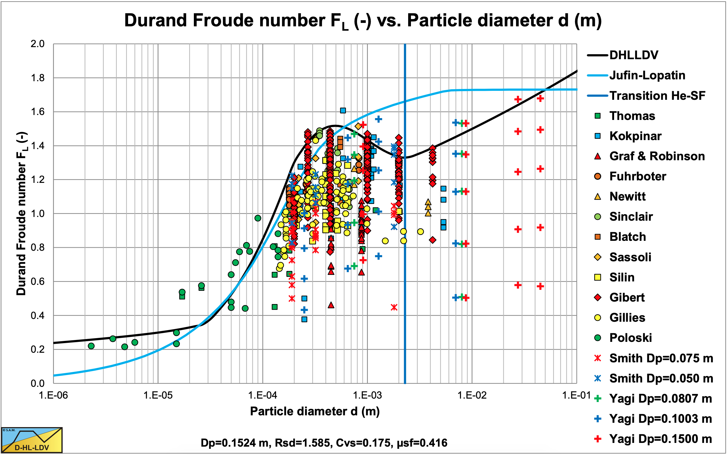
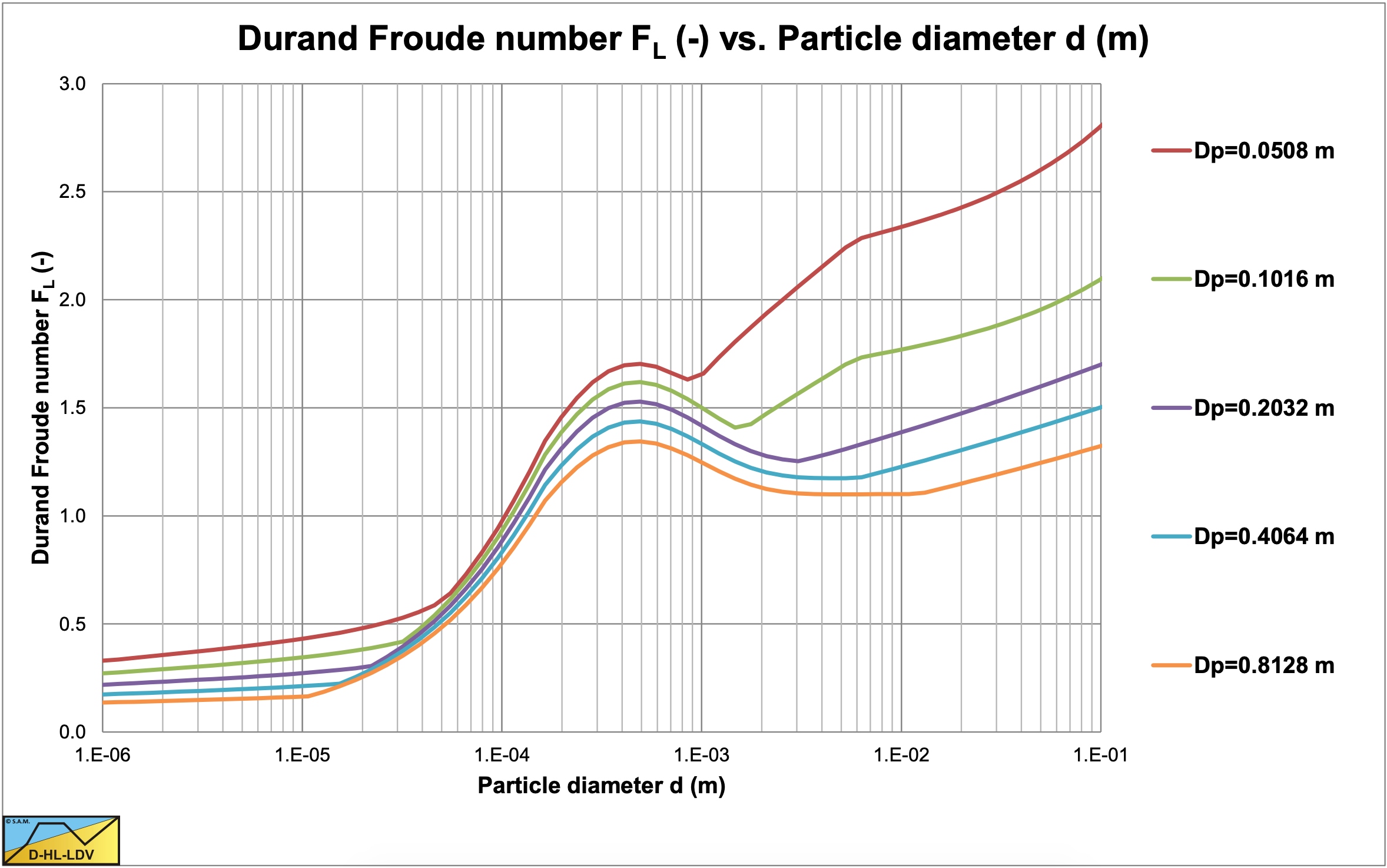
Figure 7.8-1 shows many data points of various authors for sand and gravel in water. Each column of data points shows the results of experiments with different volumetric concentrations, where the highest points were at volumetric concentrations of about 15%–20%, higher concentrations gave lower points. The experimental data also shows that smaller pipe diameters, in general, give higher Durand and Condolios (1952) Froude F_L numbers.

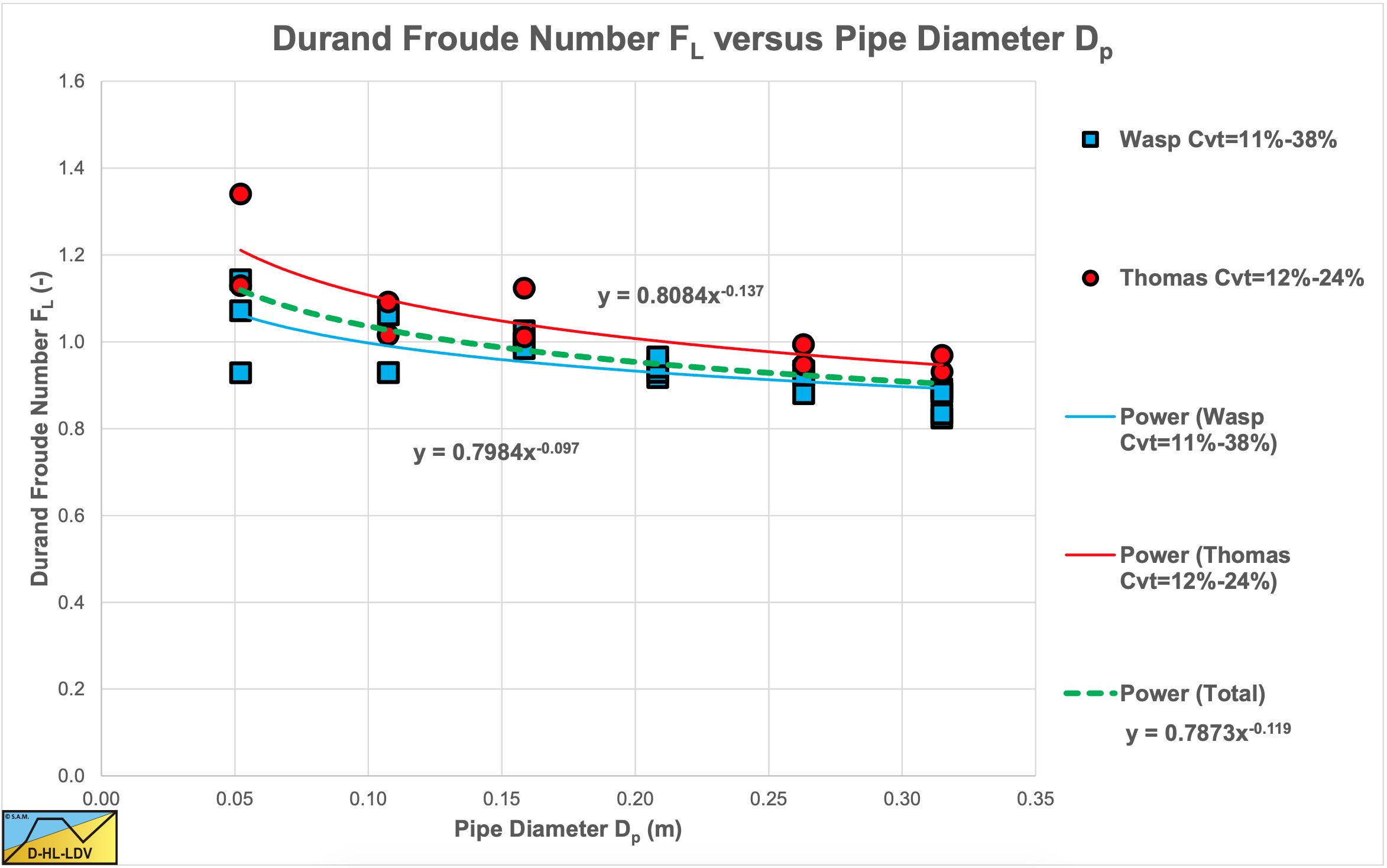
The two curves in the graph are for the Jufin and Lopatin (1966) equation, which is only valid for sand and gravel, and the DHLLDV Framework which is described in this chapter. Both models give a sort of upper limit to the LDV. The data points of the very small particle diameters, Thomas (1979) and Poloski (2010), were carried out in very small to medium diameter pipes, while the two curves are constructed for a 0.1524 (6 inch) pipe, resulting in slightly lower curves. Data points above the DHLLDV curve are in general for pipe diameters smaller than 0.1524 m. Some special attention is given to the relation between the Durand Froude F_L number and the pipe diameter D_p. Both Thomas (1979) and Wasp et al. (1977) carried out research with a d = 0.18 mm particle in 6 pipe diameters, see Figure 7.8-2. These experiments show a slight decrease of the F_L value with increasing pipe diameter with a power close to –0.1.

Figure 7.8-1: Experimental data in different pipe diameters.

Figure 7.8-2: Data of Thomas (1979) and Wasp et al. (1977) with different pipe diameters.

7.8.3 Equations & Models

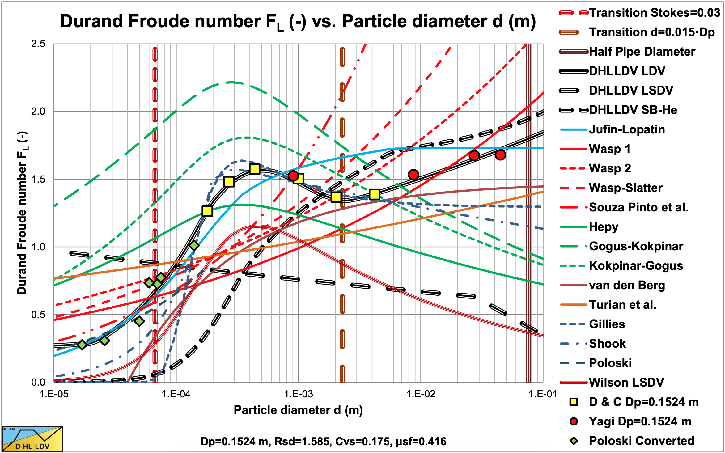
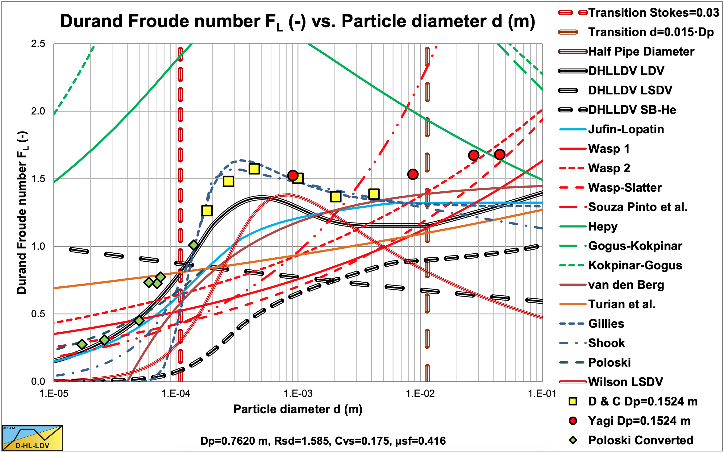
Figure 7.8-3 and Figure 7.8-4 show the Limit Deposit Velocities of DHLLDV, Durand and Condolios (1952), Jufin and Lopatin (1966), Wasp et al. (1970), Wasp and Slatter (2004), Souza Pinto et al. (2014), Hepy et al. (2008), Gogus and Kokpinar (1993), Kokpinar and Gogus (2001), Berg (1998), Turian et al. (1987) and Gillies (1993) for 2 pipe diameters. The curves of Hepy et al. (2008), Gogus and Kokpinar (1993) and Kokpinar and Gogus (2001) show a maximum F_L value for particles with a diameter near d = 0.5 mm. However these models show an increasing F_L value with the pipe diameter, which contradicts the numerous experimental data, showing a slight decrease. The models of Turian et al. (1987) , Wasp et al. (1970), Wasp and Slatter (2004) and Souza Pinto et al. (2014) show an increasing F_L value with increasing particle diameter and a slight decrease with the pipe diameter.

Jufin and Lopatin (1966) show an increase with the particle diameter and a slight decrease with the pipe diameter (power –1/6). The model of van den Berg (1998) shows an increasing F_L with the particle diameter, but no dependency on the pipe diameter. Durand and Condolios (1952) did not give an equation but a graph. The data points as derived from the original publication in (1952) and from Durand (1953) are shown in the graphs. The data points show a maximum for d = 0.5 mm. They did not report any dependency on the pipe diameter. The model of Gillies (1993) tries to quantify the Durand and Condolios (1952) data points but does not show any dependency on the pipe diameter for the F_L Froude number. The increase of the F_L value with the pipe diameter of the Hepy et al. (2008), Gogus and Kokpinar (1993) and Kokpinar and Gogus (2001) models is probably caused by the forced d/D_p relation. With a strong relation with the particle diameter and a weak relation for the pipe diameter, the pipe diameter will follow the particle diameter. Another reason may be the fact that they used pipe diameters up to 0.1524 m (6 inch) and the smaller the pipe diameter the more probable the occurrence of a sliding bed and other limiting conditions, due to the larger hydraulic gradient helping the bed to start sliding.

The figures show that for small pipe diameters all models are close. The reason is probably that most experiments are carried out with small pipe diameters. Only Jufin and Lopatin (1966) covered a range from 0.02 m to 0.9 m pipe diameters. Recently Thomas (2014) gave an overview and analysis of the LDV (or sometimes the LSDV). He repeated the findings that the LDV depends on the pipe diameter with a power smaller than 0.5 but larger than 0.1. The value of 0.1 is for very small particles, while for normal sand and gravels a power is expected between 1/3 according to Jufin and Lopatin (1966) and 1/2 according to Durand and Condolios (1952). Most equations are one term equations, making it impossible to cover all aspects of the LDV behavior. Only Gillies (1993) managed to construct an equation that gets close to the original Durand and Condolios (1952) graph.

Figure 7.8-3: A number of LDV models in a 0.1524 m (6 inch) pipe.

Figure 7.8-4: A number of LDV models in a 0.762 m (30 inch) pipe.

7.8.4 Conclusions Literature

The models analyzed result in a number of dominating parameters. These are the particle diameter d, the pipe diameter D_p, the liquid density ρ_l and kinematic viscosity ν_l, the solids density ρ_s, the sliding friction coefficient μ_sf, the bed concentration C_vb and the spatial volumetric concentration C_vs. Derived parameters are the relative submerged density R_sd, the Darcy Weisbach friction factor for pure liquid flow λ_l and the thickness of the viscous sub-layer δ_v. Dimensionless numbers are not considered at first, since they may lead to wrong interpretations. Lately Lahiri (2009) performed an analysis using artificial neural network and support vector regression. Azamathulla and Ahmad (2013) performed an analysis using adaptive neuro-fuzzy interference system and gene- expression programming. Although these methodologies may give good correlations, they do not explain the physics. Lahiri (2009) however did give statistical relations for the dependency on the volumetric concentration, the particle diameter, the pipe diameter and the relative submerged density.

Resuming, the following conclusions can be drawn for sand and gravel:
The pipe diameter D_p: The LDV is proportional to the pipe diameter D_p to a power between 1/3 and 1/2 (about 0.4) for small to large particles (Thomas (1979), Wasp et al. (1977), Lahiri (2009) and Jufin and Lopatin (1966)) and a power of about 0.1 for very small particles (Thomas (1979), Wilson and Judge (1976), Sanders et al. (2004) and Poloski et al. (2010)).
The particle diameter d: The LDV has a lower limit for very small particles, after which it increases to a maximum at a particle diameter of about d = 0.5 mm (Thomas (1979), Thomas (2014), Durand and Condolios (1952), Gillies (1993) and Poloski et al. (2010)). For medium sized particles with a particle size d > 0.5 mm, the F_L value decreases slightly to a minimum for a particle size of about d = 2 mm (Durand and Condolios, 1952; Gillies, 1993; Poloski et al., 2010). Above 2 mm, the F_L value will remain constant according to Durand and Condolios (1952) and Gillies (1993). For particles with d/D_p > 0.015, the Wilson et al. (1992) criterion for real suspension/saltation, the F_L value increases again. This criterion is based on the ratio particle diameter to pipe diameter and will start at a large particle diameter with increasing pipe diameter. Yagi et al. (1972) reported many data points in this region showing an increasing F_L value.
The relative submerged density R_sd: The relation between the LDV and the relative submerged density is not very clear, however the data shown by Kokpinar and Gogus (2001) and the conclusions of Lahiri (2009) show that the F_L value decreases with increasing solids density and thus relative submerged density R_sd to a power of –0.1 to – 0.4.
The spatial volumetric concentration C_vs: The volumetric concentration leading to the maximum LDV is somewhere between 15% and 20% according to Durand and Condolios (1952). Lahiri (2009) reported a maximum at about 17.5%, while Poloski et al. (2010) derived 15%. This maximum LDV results from on one hand a linear increase of the sedimentation with the concentration and on the other hand a reduced sedimentation due to the hindered setting. These two counteracting phenomena result in a maximum, which is also present in the equation of the potential energy. For small concentrations a minimum LDV is observed by Durand and Condolios (1952). This minimum LDV increases with the particle diameter and reaches the LDV of 20% at a particle diameter of 2 mm with a pipe diameter of 0.1524 m (6 inch).

For the dredging industry the Jufin and Lopatin (1966) equation gives a good approximation for sand and gravel, although a bit conservative. The model of Berg (1998) is suitable for large diameter pipes as used in dredging for sand and/or gravel, but underestimates the LDV for pipe diameters below 0.8 m. Both models tend to underestimate the LDV for particle diameters below 1 mm.

7.8.5 Starting Points DHLLDV Framework

Analyzing the literature, equations and experimental data, the LDV can be divided into 5 regions for sand and gravel:

1. Very small particles, smaller than about 50% of the thickness of the viscous sub layer, giving a lower limit of the LDV. This is for particles up to about 0.15 mm in large pipes to 0.04 mm in very small pipes.
2. Small particles up to about 0.2 mm, a smooth bed, show an increasing LDV with increasing particle diameter.
3. Medium particles with a diameter from 0.2 mm up to a diameter of 2 mm, a transition zone from a smooth bed to a rough bed. First the LDV increases to a particle diameter of about 0.5 mm, after which it decreases slowly to an asymptotic value at a diameter of about 2 mm.
4. Large particles with a diameter larger than 2 mm, a rough bed, giving a constant LDV.
5. Particles with a particle diameter to pipe diameter ratio larger than about 0.015 cannot be carried by turbulent eddies, just because eddies are not large enough. This will probably result in an increasing LDV with the particle diameter. Yagi et al. (1972) reported many data points in this region showing this increase.

The above conclusions are the starting points of the DHLLDV Limit Deposit Velocity Model and has been shown in the figures.

7.8.6 The Transition Fixed Bed – Sliding Bed (LSDV)

The transition fixed bed – sliding bed is not considered to be a real Limit Deposit Velocity, but it is a regime change and thus will be discussed here. This transition is named the Limit of Stationary Deposit Velocity (LSDV) resulting from 2LM or 3LM analysis like the Wilson et al. (1992) model. This transition will only occur above a certain particle diameter to pipe diameter ratio. Very small particles will never have a sliding bed. But medium sized particles that will have a sliding bed in small pipe diameters, may not have a sliding bed in large pipe diameters. Mathematically however, the transition line speed can always be determined, even though the transition will not occur in reality. In such a case the bed is already completely suspended before it could start sliding.

The total hydraulic gradient of a sliding bed i_m,sl is considered to be equal to the hydraulic gradient required to move clear liquid through the pipe i_l and the sliding friction hydraulic gradient resulting from the friction force between the solids and the pipe i_sf, is:

\[\ \mathrm{i}_{\mathrm{m}, \mathrm{s} \mathrm{b}}=\mathrm{i}_{\mathrm{l}}+\mathrm{i}_{\mathrm{s f}}=\lambda_{\mathrm{l}} \cdot \frac{\mathrm{v}_{\mathrm{l s}}^{\mathrm{2}}}{\mathrm{2} \cdot \mathrm{g} \cdot \mathrm{D}_{\mathrm{p}}}+\mu_{\mathrm{s f}} \cdot \mathrm{C}_{\mathrm{v s}} \cdot \mathrm{R}_{\mathrm{s d}}\]

The hydraulic gradient i_m,fb due to the flow through the restricted area A_H above the bed is:

\[\ \mathrm{i}_{\mathrm{m}, \mathrm{fb}}=\lambda_{\mathrm{r}} \cdot \frac{\mathrm{v}_{\mathrm{l} \mathrm{s}, \mathrm{r}}^{2}}{\mathrm{2} \cdot \mathrm{g} \cdot \mathrm{D}_{\mathrm{H}}}=\lambda_{\mathrm{r}} \cdot \frac{\mathrm{v}_{\mathrm{l s}}^{2}}{2 \cdot \mathrm{g} \cdot \mathrm{D}_{\mathrm{H}}} \cdot\left(\frac{\mathrm{A}_{\mathrm{p}}}{\mathrm{A}_{\mathrm{H}}}\right)^{\mathrm{2}}\]

This gives for the transition line speed:

\[\ \mathrm{v}_{\mathrm{ls}, \mathrm{FBSB}}^{2}=\frac{2 \cdot \mu_{\mathrm{sf}} \cdot \mathrm{g} \cdot \mathrm{C}_{\mathrm{vs}} \cdot \mathrm{R}_{\mathrm{sd}}}{\frac{\lambda_{\mathrm{r}}}{\mathrm{D}_{\mathrm{H}}} \cdot\left(\frac{\mathrm{A}_{\mathrm{p}}}{\mathrm{A}_{\mathrm{H}}}\right)^{2}-\frac{\lambda_{\mathrm{l}}}{\mathrm{D}_{\mathrm{p}}}}\]

7.8.7 The Transition Heterogeneous – Homogeneous (LDV Very Fine Particles)

For very fine particles, the Limit Deposit Velocity is close to the transition between the heterogeneous regime and the homogeneous regime. Values found in literature (Thomas (1976)) are between 80% and 100% of this transition velocity. This transition velocity can be determined by making the relative excess pressure contributions of both regimes equal, according to:

\[\ \mathrm{R}_{\mathrm{sd}} \cdot \mathrm{C}_{\mathrm{v s}}=\frac{\left(\mathrm{2} \cdot \mathrm{g} \cdot \mathrm{R}_{\mathrm{s d}} \cdot \mathrm{D}_{\mathrm{p}}\right)}{\lambda_{\mathrm{l}}} \cdot \mathrm{C}_{\mathrm{v s}} \cdot \frac{\mathrm{1}}{\mathrm{v}_{\mathrm{l s}}^{2}} \cdot\left(\frac{\mathrm{v}_{\mathrm{t}}}{\mathrm{v}_{\mathrm{l s}}} \cdot\left(\mathrm{1}-\frac{\mathrm{C}_{\mathrm{v s}}}{\mathrm{\kappa}_{\mathrm{C}}}\right)^{\beta}+\frac{\mathrm{8.5}^{2}}{\lambda_{\mathrm{l}}} \cdot\left(\frac{\mathrm{v}_{\mathrm{t}}}{\sqrt{\mathrm{g} \cdot \mathrm{d}}}\right)^{\mathrm{1 0 / 3}} \cdot\left(\frac{\left(v_{\mathrm{l}} \cdot \mathrm{g}\right)^{1 / 3}}{\mathrm{v}_{\mathrm{l s}}}\right)^{2}\right)\]

This gives for the transition velocity between the heterogeneous regime and the homogeneous regime:

\[\ \mathrm{v}_{\mathrm{ls}, \mathrm{HeHo}}^{4}=\frac{2 \cdot \mathrm{g} \cdot \mathrm{D}_{\mathrm{p}}}{\lambda_{\mathrm{l}}} \cdot\left(\mathrm{v}_{\mathrm{t}} \cdot\left(1-\frac{\mathrm{C}_{\mathrm{vs}}}{\kappa_{\mathrm{C}}}\right)^{\beta} \cdot \mathrm{v}_{\mathrm{ls}, \mathrm{HeHo}}+\frac{8.5^{2}}{\lambda_{\mathrm{l}}} \cdot\left(\frac{\mathrm{v}_{\mathrm{t}}}{\sqrt{\mathrm{g} \cdot \mathrm{d}}}\right)^{10 / 3} \cdot\left(v_{\mathrm{l}} \cdot \mathrm{g}\right)^{2 / 3}\right)\]

This equation implies that the transition line speed depends reversely on the Darcy Weisbach viscous friction coefficient λ_l. Since the viscous friction coefficient λ_l depends reversely on the pipe diameter D_p with a power of about 0.2, the transition line speed will depend on the pipe diameter with a power of about (1.2/4) =0.3. It is advised to use the Thomas (1965) viscosity correction for this transition line speed, otherwise to high transition velocities may be found. The equation derived is implicit and has to be solved iteratively.

7.8.8 The Transition Sliding Bed – Heterogeneous (LDV Coarse Particles)

When a sliding bed is present, particles will be in suspension above the sliding bed. The higher the line speed, the more particles will be in suspension. The interaction between the particles in suspension and the particles in the bed will still be by inter particle interactions, reason that the sliding bed is still carrying the weight of all the particles in suspension. Apparently the weight of all the particles is resulting in sliding friction. At a certain line speed all the particles will be in suspension and the sliding bed regime transits to heterogeneous flow. The particles now interact with the pipe wall by collisions and not by sliding friction anymore.

At the transition line speed the excess pressure losses of both regimes should be equal, giving

\[\ \mu_{\mathrm{sf}}=\frac{\mathrm{v}_{\mathrm{t}}}{\mathrm{v}_{\mathrm{ls}}} \cdot\left(1-\frac{\mathrm{C}_{\mathrm{vs}}}{\kappa_{\mathrm{C}}}\right)^{\beta}+\frac{8.5^{2}}{\lambda_{\mathrm{l}}} \cdot\left(\frac{\mathrm{v}_{\mathrm{t}}}{\sqrt{\mathrm{g} \cdot \mathrm{d}}}\right)^{10 / 3} \cdot\left(\frac{(v \cdot \mathrm{g})^{1 / 3}}{\mathrm{v}_{\mathrm{ls}}}\right)^{2}\]

Resulting in the transition velocity at:

\[\ \mathrm{v}_{\mathrm{l s}, \mathrm{S B H e}}^{2}=\frac{\mathrm{v}_{\mathrm{t}} \cdot(\mathrm{1 - \frac { \mathrm { C } _ { \mathrm { v s } } } { \mathrm { \kappa } _ { \mathrm { C } } }})^{\beta} \cdot \mathrm{v}_{\mathrm{l s}, \mathrm{S B H e}}+\frac{\mathrm{8 . 5}^{\mathrm{2}}}{\lambda_{\mathrm{l}}} \cdot\left(\frac{\mathrm{v}_{\mathrm{t}}}{\sqrt{\mathrm{g} \cdot \mathrm{d}}}\right)^{\mathrm{1 0 / 3}} \cdot\left(v_{\mathrm{l}} \cdot \mathrm{g}\right)^{2 / 3}}{\boldsymbol{\mu}_{\mathrm{s f}}}\]

This equation shows that the transition between the sliding bed regime and the heterogeneous regime depends on the sliding friction coefficient. Implicitly Newitt et al. (1955) already found this, but didn’t explicitly mention this, because they assumed that potential energy is responsible for all the excess head losses in heterogeneous flow. The equation derived is a second degree function and can be written as:

\[\ \mathrm{-v_{ls,SBHe}^2+\frac{v_t \cdot \left(1-\frac{C_{vs}}{\kappa_C} \right)^{\beta}}{\mu_{sf}}\cdot v_{ls,SBHe}}+\frac{\frac{8.5^2}{\lambda_\mathrm{l}}\cdot \left(\frac{\mathrm{v_t}}{\sqrt{\mathrm{g \cdot d} }} \right)^{10/3}\cdot (v_{\mathrm{l}\cdot \mathrm{g}})^{2/3}}{\mu_{\mathrm{sf}}}=0 \]

With:

\[\ \begin{array}{left} \mathrm{A} =-1\\
\mathrm{B =\frac{v_{t} \cdot\left(1-\frac{C_{v s}}{\kappa_{C}}\right)^{\beta}}{\mu_{s f}}}\\
\mathrm{C}=\frac{\frac{8.5^{2}}{\lambda_{\mathrm{l}}} \cdot\left(\frac{\mathrm{v_{t}}}{\sqrt{\mathrm{g \cdot d}}}\right)^{10 / 3} \cdot\left(v_{\mathrm{l}} \cdot \mathrm{g}\right)^{2 / 3}}{\mu_{s f}} \\ \mathrm{v_{\mathrm{ls}, \mathrm{SBHe}}=\frac{-B-\sqrt{B^{2}-4 \cdot A \cdot C}}{2 \cdot A}}\end{array}
\]

The lower limit of the LDV is found to be about 80% of this transition line speed. This also implies that the transition of a sliding bed to heterogeneous transport is not sharp, an intersection point, but it’s a gradual process starting at about 80% of the transition line speed.

7.8.9 The Transition Sliding Bed – Homogeneous (LSBV)

The transition sliding bed – homogeneous is not considered to be a Limit Deposit Velocity here, because for normal dredging operations this is out of range.
The total hydraulic gradient of a sliding bed i_m,sl is considered to be equal to the hydraulic gradient required to move clear liquid through the pipe i_l and the sliding friction hydraulic gradient resulting from the friction force between the solids and the pipe i_sf, is:

\[\ \mathrm{i}_{\mathrm{m}, \mathrm{sb}}=\mathrm{i}_{\mathrm{l}}+\mathrm{i}_{\mathrm{s f}}=\lambda_{\mathrm{l}} \cdot \frac{\mathrm{v}_{\mathrm{l s}}^{2}}{2 \cdot \mathrm{g} \cdot \mathrm{D}_{\mathrm{p}}}+\mu_{\mathrm{s f}} \cdot \mathrm{C}_{\mathrm{v s}} \cdot \mathrm{R}_{\mathrm{s d}}\]

The total hydraulic gradient of homogeneous flow according to the ELM model is:

\[\ \begin{array}{left} \mathrm{i}_{\mathrm{m}, \mathrm{h} \mathrm{o}}&=\mathrm{i}_{\mathrm{l}}+\mathrm{i}_{\mathrm{s}}=\lambda_{\mathrm{l}} \cdot \frac{\mathrm{v}_{\mathrm{l} \mathrm{s}}^{\mathrm{2}}}{\mathrm{2} \cdot \mathrm{g} \cdot \mathrm{D}_{\mathrm{p}}} \cdot\left(\mathrm{1}+\mathrm{R}_{\mathrm{s} \mathrm{d}} \cdot \mathrm{C}_{\mathrm{v s}}\right)\\
&=\lambda_{\mathrm{l}} \cdot \frac{\mathrm{v}_{\mathrm{l} \mathrm{s}}^{2}}{\mathrm{2} \cdot \mathrm{g} \cdot \mathrm{D}_{\mathrm{p}}}+\lambda_{\mathrm{l}} \cdot \frac{\mathrm{v}_{\mathrm{l} \mathrm{s}}^{2}}{\mathrm{2} \cdot \mathrm{g} \cdot \mathrm{D}_{\mathrm{p}}} \cdot \mathrm{R}_{\mathrm{s} \mathrm{d}} \cdot \mathrm{C}_{\mathrm{v} \mathrm{s}}\end{array}\]

At the transition velocity both are equal giving:

\[\ \mu_{\mathrm{sf}}=\lambda_{\mathrm{l}} \cdot \frac{\mathrm{v}_{\mathrm{ls}}^{2}}{2 \cdot \mathrm{g} \cdot \mathrm{D}_{\mathrm{p}}}\]

So the transition velocity is:

\[\ \mathrm{v}_{\mathrm{l} \mathrm{s}, \mathrm{s} \mathrm{b}-\mathrm{h o}}^{2}=\frac{\mathrm{2} \cdot \boldsymbol{\mu}_{\mathrm{s f}} \cdot \mathrm{g} \cdot \mathrm{D}_{\mathrm{p}}}{\lambda_{\mathrm{l}}}\]

7.8.10 The Limit Deposit Velocity (LDV All Particles)

7.8.10.1 Introduction

Before starting with the derivation of the model two phenomena will be discussed, supporting the philosophy behind the model. First the turbulent velocity distribution above a bed, ranging from a very smooth bed to a very rough bed. Second the suspension criterion from the Shields-Parker diagram.

In the turbulent layer the total shear stress contains only the turbulent shear stress. Integration of the shear stress gives the famous logarithmic velocity profile (Law of the Wall):

\[\ \mathrm{u}(\mathrm{y})=\frac{\mathrm{u}_{*}}{\mathrm{\kappa}} \cdot \ln \left(\frac{\mathrm{y}}{\mathrm{y}_{\mathrm{0}}}\right)\]

Where the integration constant y₀ is the elevation corresponding to zero velocity (u_y=y₀=0), given by Nikuradse by the study of the pipe flows.

\[\ \mathrm{y}_{0}=\mathrm{0 .1 1} \cdot \frac{v_{1}}{\mathrm{u}_{*}} \quad\text{ Hydraulically smooth flow }\quad \frac{\mathrm{u}_{*} \cdot \mathrm{k}_{\mathrm{s}}}{v_{\mathrm{l}}} \leq \mathrm{5}\]

\[\ \mathrm{y}_{0}=\mathrm{0 .0 3 3} \cdot \mathrm{k}_{\mathrm{s}} \quad\text{ Hydraulically rough flow} \quad
\frac{\mathrm{u}_{*} \cdot \mathrm{k}_{\mathrm{s}}}{v_{\mathrm{l}}} \geq 7 \mathrm{0}\]

\[\ \frac{\mathrm{y}_{0}}{\mathrm{k}_{\mathrm{s}}}=\frac{1}{\mathrm{9} \cdot \mathrm{k}_{\mathrm{s}}^{+}}+\frac{\mathrm{1}}{\mathrm{3 0}} \cdot\left(\mathrm{1}-\mathrm{e}^{-\frac{\mathrm{k}_{\mathrm{s}}^{+}}{\mathrm{2 6}}}\right) \quad\text{ Hydraulically transition flow }\quad \mathrm{5}<\frac{\mathrm{u}_{*} \cdot \mathrm{k}_{\mathrm{s}}}{v_{\mathrm{l}}}<\mathrm{7 0}\]

Figure 7.8-5: The transition smooth-rough for a number of distances to the wall.

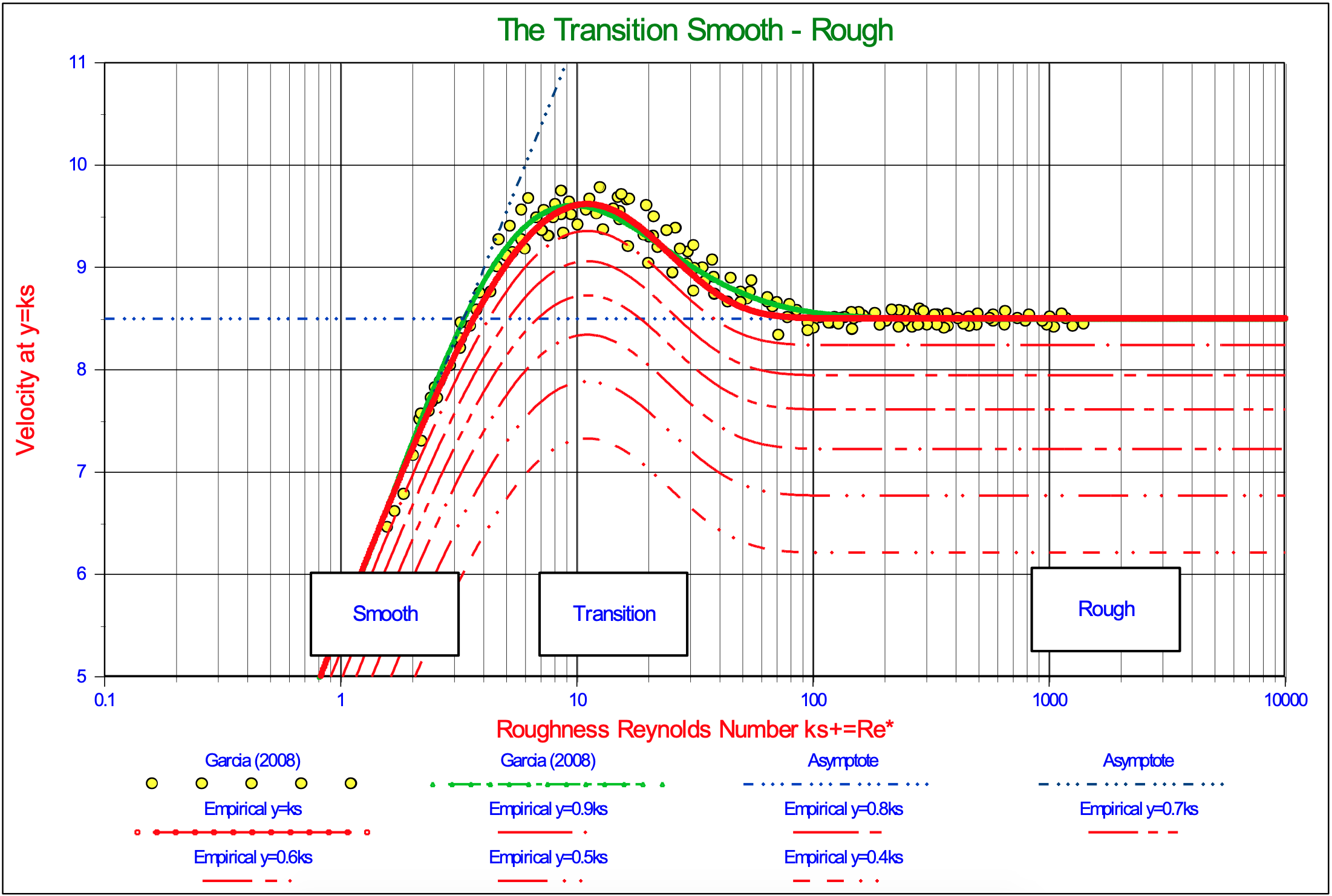
The transition between hydraulic smooth and rough flow can be approximated in many ways, but the resulting equation should match measurements like shown in Garcia (2008) (fig. 2.3). The following equation (derived by the Miedema (2012A)), gives a very good approximation of this transition, where the distance to the wall equals the roughness. Equation (7.8-25) gives the velocity as a function of the non-dimensional distance to the wall y⁺.

\[\ \frac{\overline{\mathrm{u}}\left(\mathrm{y}^{+}\right)}{\mathrm{u}_{*}}=\frac{\mathrm{1}}{\mathrm{\kappa}} \cdot \ln \left(\frac{\mathrm{y}^{+}}{\mathrm{0 .11}}\right) \cdot \mathrm{e}^{-\mathrm{0 . 9 5} \cdot \frac{\mathrm{k}_{\mathrm{s}}^{+}}{11.6}}+\frac{\mathrm{1}}{\mathrm{\kappa}} \cdot \ln \left(\frac{\mathrm{y}^{+}}{\mathrm{0.033} \cdot \mathrm{k}_{\mathrm{s}}^{+}}\right) \cdot\left(1-\mathrm{e}^{-\mathrm{0 . 9 5} \cdot \frac{\mathrm{k}_{\mathrm{s}}^{+}}{11.6}}\right)\]

Since \(\ \mathrm{1 1 .6}=\delta_{\mathrm{v}} \cdot \mathrm{u}_{*} / v=\delta_{\mathrm{v}}^{+}\text{ and }\mathrm{0.11}=\mathrm{0.11} \cdot \delta_{\mathrm{v}} \cdot \mathrm{u}_{*} / v / \mathrm{11 .6}=\mathrm{0.0095} \cdot \delta_{\mathrm{v}}^{+}\) and the influence of the second right hand term (giving 95 instead of 105), equation (5.1-20) can be written as:

\[\ \frac{\overline{\mathrm{u}}\left(\mathrm{y}^{+}\right)}{\mathrm{u}_{*}}=\frac{\mathrm{1}}{\mathrm{\kappa}} \cdot \ln \left(\mathrm{9 5} \cdot \frac{\mathrm{y}^{+}}{\delta_{\mathrm{v}}^{+}}\right) \cdot \mathrm{e}^{-0.95 \cdot \frac{\mathrm{k}_{s}^{+}}{\delta_{v}^{+}}}+\frac{\mathrm{1}}{\mathrm{\kappa}} \cdot \ln \left(\mathrm{3 0} \cdot \frac{\mathrm{y}^{+}}{\mathrm{k}_{\mathrm{s}}^{+}}\right) \cdot\left(1-\mathrm{e}^{-0.95 \cdot \frac{\mathrm{k}_{s}^{+}}{\delta_{v}^{+}}}\right)\]

In terms of the dimensional parameters for the distance to the wall y, the roughness k_s and thickness of the laminar layer δ_v this gives:

\[\ \frac{\overline{\mathrm{u}}(\mathrm{y})}{\mathrm{u}_{*}}=\frac{\mathrm{1}}{\mathrm{\kappa}} \cdot \ln \left(\mathrm{9 5} \cdot \frac{\mathrm{y}}{\delta_{\mathrm{v}}}\right) \cdot \mathrm{e}^{-\mathrm{0.95} \cdot \frac{\mathrm{k}_{\mathrm{s}}}{\delta_{\mathrm{v}}}}+\frac{\mathrm{1}}{\mathrm{\kappa}} \cdot \ln \left(\mathrm{3 0} \cdot \frac{\mathrm{y}}{\mathrm{k}_{\mathrm{s}}}\right) \cdot\left(1-\mathrm{e}^{-0.95 \cdot \frac{\mathrm{k}_{\mathrm{s}}}{\delta_{\mathrm{v}}}}\right)\]

Figure 7.8-5 shows the non-dimensional velocity u⁺ at distances y=k_s, y=0.9k_s, y=0.8k_s, y=0.7k_s, y=0.6k_s, y=0.5k_s and, y=0.4k_s from the wall. Up to a Reynolds number of 20 and above a Reynolds number of 70 equation (7.8-27) matches the measurements very well, between 20 and 70 the equation underestimates the measured values, but overall the resemblance is very good.

Figure 7.8-5 shows a shape of the curves similar to the shape of the LDV curve as reported by Durand & Condolios (1952).

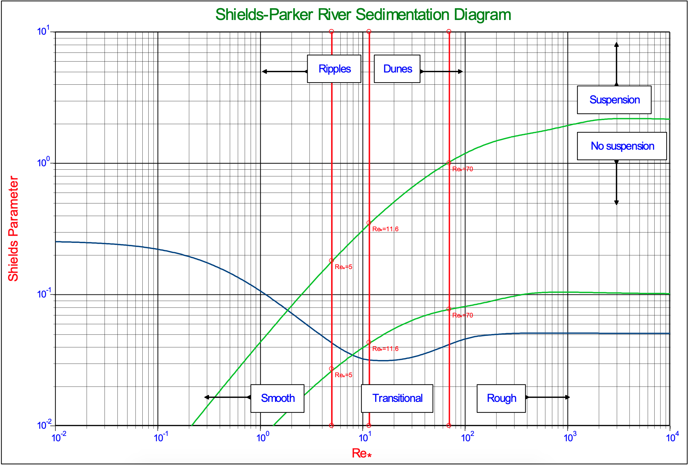
A well-known application of the Shields curve is the so called Shields-Parker diagram, showing erosion versus no erosion, suspension versus no suspension and ripples versus dunes. This diagram is shown in Figure 7.8-6. The criterion used for the suspension curve is:

\[\ \mathrm{v}_{\mathrm{t}}=\mathrm{u}_{*}\]

The terminal settling velocity equals the friction velocity. Now this is not an absolute criterion, much more an indication.

At a point Re_*=2 and θ=0.08 the suspension curve crosses the Shields curve. At smaller Reynolds numbers the suspension curve is lower than the Shields curve. For sand this intersection point is for particles with d=0.146 mm. Physically this means that particles smaller than d=0.146 mm once in suspension will stay in suspension even if the Shields number is below the Shields curve. However if there is some bed, a much higher line speed is required to erode the bed, because the bed is very smooth. Whether or not a bed will be present depends on the history. If the line speed is gradually increased starting from zero, there will be a bed and a relatively high line speed is required to erode the bed. However, if the line speed is gradually decreased starting with a very high line speed, all particles will be in suspension and remain in suspension until the line speed is low enough.

Figure 7.8-6: The Shields-Parker diagram as a function of the roughness Reynolds number Re_*.

7.8.10.2 Very Small Particles, the Lower Limit

Thomas (1979) investigated the Limit Deposit Velocity for very small particles and found that there is a lower limit to the LDV independent of the particle size. According to Figure 7.8-6 this occurs for particles smaller than d=0.146 mm, although this is just an indication. This lower limit is based on the assumption that the very small particles are smaller than the thickness of the viscous sub layer and still settle in this laminar flow, while particles in the turbulent flow are carried by the small eddies. At the moment of sliding the shear stress \(\ \tau_{12} \) at the top of the thin layer with thickness h, equals the sliding friction force divided by the total sliding surface:

\[\ \tau_{12}=\frac{\mathrm{F_{\mathrm{sf}}}}{\mathrm{D}_{\mathrm{p}} \cdot \Delta \mathrm{L}}=\mu_{\mathrm{sf}} \cdot \mathrm{h} \cdot \rho_{\mathrm{l}} \cdot \mathrm{R}_{\mathrm{sd}} \cdot(1-\mathrm{n}) \cdot \mathrm{g}=\mu_{\mathrm{sf}} \cdot \mathrm{h} \cdot \rho_{\mathrm{l}} \cdot \mathrm{R}_{\mathrm{sd}} \cdot \mathrm{C}_{\mathrm{vb}} \cdot \mathrm{g}\]

The thickness of the thin layer is assumed to be equal to the thickness of the viscous sub layer:

\[\ \mathrm{h}=\delta_{\mathrm{v}}=\mathrm{11.6} \cdot \frac{v_{\mathrm{l}}}{\mathrm{u}_{*}}\]

Thomas (1979) used a factor 5 instead of 11.6. Substituting this layer thickness gives:

\[\ \tau_{12}=11.6 \cdot \mu_{\mathrm{sf}} \cdot \frac{v_{1}}{\mathrm{u}_{*}} \cdot \rho_{\mathrm{l}} \cdot \mathrm{R}_{\mathrm{sd}} \cdot \mathrm{C}_{\mathrm{vb}} \cdot \mathrm{g}=\rho_{\mathrm{l}} \cdot \mathrm{u}_{*}^{2}\]

This gives for the friction velocity:

\[\ \mathrm{u}_{*}^{\mathrm{3}}=\mathrm{11.6} \cdot \mu_{\mathrm{s f}} \cdot v_{\mathrm{l}} \cdot \mathrm{R}_{\mathrm{s d}} \cdot \mathrm{C}_{\mathrm{v b}} \cdot \mathrm{g} \quad\text{ or }\quad \mathrm{u}_{*}=\mathrm{2.2 6} \cdot\left(\mu_{\mathrm{s f}} \cdot v_{\mathrm{l}} \cdot \mathrm{R}_{\mathrm{s d}} \cdot \mathrm{C}_{\mathrm{v b}} \cdot \mathrm{g}\right)^{1 / 3}\]

With a bed concentration C_vb=0.6 and a sliding friction coefficient of μ_sf=0.4 this gives:

\[\ \mathrm{u}_{*}=\mathrm{1 . 4} \cdot\left(v_{\mathrm{l}} \cdot \mathrm{R}_{\mathrm{s d}} \cdot \mathrm{g}\right)^{1 / 3} \quad\text{ or }\quad \mathrm{u}_{*}=\mathrm{0.0 3 8 7}\]

For sand with a relative submerged density of R_sd=1.65, water with a viscosity of ν_l=0.0000013 m²/sec this gives a friction velocity of 0.0387 m/sec. In terms of the Limit Deposit Velocity the following is found:

\[\ \begin{array}{left} \mathrm{u}_{*}=\sqrt{\frac{\lambda_{\mathrm{l}}}{\mathrm{8}}}{ \cdot \mathrm{v}_{\mathrm{l} \mathrm{s}, \mathrm{l} \mathrm{d} \mathrm{v}}=\mathrm{1 .4} \cdot\left(v_{\mathrm{l}} \cdot \mathrm{R}_{\mathrm{s d}} \cdot \mathrm{g}\right)^{1 / \mathrm{3}}} \quad\text{ or }\quad \mathrm{u}_{*}=\sqrt{\frac{\lambda_{\mathrm{l}}}{\mathrm{8}}}{ \cdot \mathrm{v}_{\mathrm{l} \mathrm{s}, \mathrm{l d v}}=\mathrm{0} . \mathrm{0 3 8 7}}\\ \mathrm{v_{\mathrm{l s}, \mathrm{l d v}}}=1 .4 \cdot ( v _ \mathrm{l} {\cdot \mathrm { R } _ { \mathrm { s d } } \cdot \mathrm { g } ) ^ { 1 / 3 } \cdot \sqrt { \frac { \mathrm { 8 } } { \lambda _ { \mathrm { l } } } }} \quad\text{ or }\quad \mathrm{v}_{\mathrm{l s}, \mathrm{l d v}}=\mathrm{0 . 0 3 8 7} \cdot \sqrt{\frac{\mathrm{8}}{\lambda_{\mathrm{l}}}} \\
\mathrm{v_{ls,ldv}}=3.96 \cdot \frac{(v_{\mathrm{l}} \cdot \mathrm{R_{sd}\cdot g})^{1/3}}{\sqrt{\lambda_{\mathrm{l}}}} \text{ or } \mathrm{v_{ls,ldv}=0.11 \cdot \sqrt{\frac{1}{\lambda_{l}}}} \end{array}\]

For small pipes with λ_l=0.03 this gives v_ls,ldv=0.64 m/sec, for medium pipes with λ_l=0.02 this gives v_ls,ldv=0.78 m/sec and for large pipe diameters with λ_l=0.01 this gives v_ls,ldv=1.10 m/sec. The LDV increases with the pipe diameter to a power of about 0.1 as already noted by Thomas (1979). Because Thomas (1979) used a factor 5 for the thickness of the viscous sub layer instead of the 11.6 as used here, he found a theoretical coefficient of 0.933 instead of the coefficient 1.4 found here. Based on his experiments he corrected this factor to 1.1. Now the value of the thickness of the viscous sub layer is just a mathematical thickness, so it is very well possible that the thickness as used here is smaller than the one using the coefficient of 11.6 and larger than using the coefficient of 5. Based on the experimental coefficient of 1.1 as found by Thomas (1979) the coefficient for the thickness of the viscous sub layer involved should be 5.62, almost 50% of the thickness of the viscous sub layer. It should be noted that the velocity found this way is in fact the LSDV and not the LDV. The LSDV is the Limit of Stationary Deposit, so the line speed where the bed starts sliding, while the LDV is the Limit Deposit Velocity, the line speed where all particles are in suspension and there is also no sliding bed anymore. The LDV is always higher than the LSDV. However it is the question whether for very small particles residing in the viscous sub layer, the situation of having 100% of the particles in suspension will ever occur. Another issue is the apparent viscosity. As the volumetric concentration increases, so does the apparent viscosity for very small particles, according to Thomas (1965). To include the viscosity effect and to be on the safe side, the factor 1.4 is used in the DHLLDV Framework.

In terms of the Durand & Condolios Froude number this gives:

\[\ \mathrm{F}_{\mathrm{L}}=\frac{\mathrm{v}_{\mathrm{ls}, \mathrm{ld v}}}{\sqrt{\mathrm{2} \cdot \mathrm{g} \cdot \mathrm{R}_{\mathrm{s d}} \cdot \mathrm{D}_{\mathrm{p}}}}=\mathrm{3.9 6} \cdot \frac{\left(v_{\mathrm{l}} \cdot \mathrm{R}_{\mathrm{s d}} \cdot \mathrm{g}\right)^{1 / 3}}{\sqrt{\lambda_{\mathrm{l}}} \cdot \sqrt{\mathrm{2} \cdot \mathrm{g} \cdot \mathrm{R}_{\mathrm{s d}} \cdot \mathrm{D}_{\mathrm{p}}}} \approx \frac{\mathrm{0 . 0 2}}{\sqrt{\lambda_{\mathrm{l}} \cdot \mathrm{D}_{\mathrm{p}}}}\]

7.8.10.3 Smooth Bed

Small particles are kept in suspension by the turbulent eddies if there is enough turbulent energy in the liquid flow. This will of course only be valid for particles small enough to be carried by these eddies. The potential energy losses of the particles are decreasing with increasing line speed, while the energy losses of the liquid flow are increasing with increasing line speed. Now it is assumed that a certain fraction of the energy losses of the liquid flow is available for the suspension of the particles. This fraction is defined as 1/α_p³. So at the line speed where the potential energy losses are equal to 1/α_p³ times the liquid energy losses, all particles will be in suspension. At a lower line speed some particles will form a bed at the bottom of the pipe. The potential energy losses of the particles can be expressed by means of the excess hydraulic gradient due to potential energy. The liquid flow energy losses can be expressed in terms of the liquid hydraulic gradient. This gives:

\[\ \frac{\mathrm{v}_{\mathrm{t}} \cdot\left(\mathrm{1}-\frac{\mathrm{C}_{\mathrm{v} \mathrm{s}}}{\mathrm{\kappa}_{\mathrm{C}}}\right)^{\beta} \cdot \mathrm{C}_{\mathrm{v} \mathrm{s}} \cdot \mathrm{R}_{\mathrm{s} \mathrm{d}}}{\mathrm{v}_{\mathrm{l} \mathrm{s}, \mathrm{l} \mathrm{d} \mathrm{v}}}=\frac{\mathrm{1}}{\mathrm{\alpha}_{\mathrm{p}}^{3}} \cdot \frac{\lambda_{\mathrm{l}} \cdot \mathrm{v}_{\mathrm{l} \mathrm{s}, \mathrm{ld} \mathrm{v}}^{2}}{\mathrm{2} \cdot \mathrm{g} \cdot \mathrm{D}_{\mathrm{p}}}\]

This gives for the Limit Deposit Velocity:

\[\ \mathrm{v}_{\mathrm{ls}, \mathrm{ldv}}^{3}=\alpha_{\mathrm{p}}^{3} \cdot \frac{\mathrm{v}_{\mathrm{t}} \cdot\left(1-\frac{\mathrm{C}_{\mathrm{vs}}}{\mathrm{\kappa}_{\mathrm{C}}}\right)^{\beta} \cdot \mathrm{C}_{\mathrm{vs}} \cdot\left(2 \cdot \mathrm{g} \cdot \mathrm{R}_{\mathrm{sd}} \cdot \mathrm{D}_{\mathrm{p}}\right)}{\lambda_{\mathrm{l}}}\]

This equation shows that the Limit Deposit Velocity of small particles depends on the terminal settling velocity with a correction for hindered settling v_t·(1-C_vs/κ_C)^β, the spatial volumetric concentration C_vs, the relative submerged density R_sd, the pipe diameter D_p and the Darcy Weisbach friction factor λ_l. The term (1-C_vs/κ_C)^β·C_v has a maximum at a spatial concentration of 15% for small particles and at about 20-25% for large particles, depending on the value of the power β and the factor κ_C. In terms of the Durand & Condolios LDV Froude number F_L factor this can be written as:

\[\ \begin{array}{left} \mathrm{F}_{\mathrm{L}, \mathrm{s}}=\frac{\mathrm{v}_{\mathrm{l s}, \mathrm{ld v}}}{\left(2 \cdot \mathrm{g} \cdot \mathrm{R}_{\mathrm{s d}} \cdot \mathrm{D}_{\mathrm{p}}\right)^{1 / 2}}=\alpha_{\mathrm{p}} \cdot\left(\frac{\mathrm{v}_{\mathrm{t}} \cdot\left(\mathrm{1}-\frac{\mathrm{C}_{\mathrm{v} \mathrm{s}}}{\mathrm{\kappa}_{\mathrm{C}}}\right)^{\beta} \cdot \mathrm{C}_{\mathrm{v s}}}{\lambda_{\mathrm{l}} \cdot\left(\mathrm{2} \cdot \mathrm{g} \cdot \mathrm{R}_{\mathrm{s d}} \cdot \mathrm{D}_{\mathrm{p}}\right)^{1 / 2}}\right)^{1 / 3}\\ \text{with: }\quad \alpha_{\mathrm{p}}=3.4 \cdot\left(\frac{\mathrm{1 .6 5}}{\mathrm{R}_{\mathrm{s d}}}\right)^{2 / 9}, \quad \kappa_{\mathrm{C}}=\mathrm{0 .1 7 5} \cdot(\mathrm{1}+\beta)\end{array}\]

The values found for α_p=3.4 and κ_C=0.175*(1+β) are based on many experiments from literature. The value of α_p of 3.4 found shows that the LDV occurs when the potential energy losses of the particles are about 2.54% of the energy losses of the liquid flow for small particles. The value of κ_C means that the average particle is at 0.175*(1+β) of the radius of the pipe, measured from the bottom of the pipe and not at the radius. This is in fact the concentration eccentricity factor. It also appears that the Limit Deposit Velocity found for small particles is close to the transition between the heterogeneous regime and the homogeneous regime, which makes sense, because in the homogeneous regime all particles are supposed to be in suspension.

The value of α_p=3.4 is based on the maximum LDV values found in literature and not on a best fit. In fact α_p may vary from 3.0 as a lower limit to 3.4 as an upper limit. So the value of 3.4 is conservative. A best fit would probably give a value of about 3.2. However in dredging the LDV should be a safe LDV, since the particle size, the concentration and the line speed may vary in time.

7.8.10.4 Rough Bed

When the particles are larger, the small eddies are not strong enough to keep them in suspension. The transport mechanism over the bottom of the pipe will be more saltation or similar to sheet flow. For medium and large particles in sedimentation transport it is often assumed that particles are in suspension or in saltation when the friction velocity is larger than the terminal settling velocity, u*>v_t. Larger particles will be more difficult to keep in suspension, but at a certain bed shear stress saltation will take over. Whether this occurs exactly at u*=v_t can be questioned, but some proportionality seems reasonable since the friction velocity is proportional to the bed shear stress. The Shields-Parker diagram, Figure 7.8-6, (Garcia, 2008), uses this assumption. Substituting the friction velocity for the terminal settling velocity gives:

\[\ \frac{\mathrm{u}_{*} \cdot\left(\mathrm{1}-\frac{\mathrm{C}_{\mathrm{v} \mathrm{s}}}{\mathrm{\kappa}_{\mathrm{C}}}\right)^{\beta} \cdot \mathrm{C}_{\mathrm{v} \mathrm{s}} \cdot \mathrm{R}_{\mathrm{s} \mathrm{d}}}{\mathrm{v}_{\mathrm{l} \mathrm{s}, \mathrm{ldv}}}=\frac{\mathrm{1}}{\alpha_{\mathrm{p}}^{3}} \cdot \frac{\lambda_{\mathrm{l}} \cdot \mathrm{v}_{\mathrm{l} \mathrm{s}, \mathrm{ldv}}^{2}}{\mathrm{2} \cdot \mathrm{g} \cdot \mathrm{D}_{\mathrm{p}}}\]

The question is now, what to use for the friction velocity u*? In general a limiting volumetric bed concentration can be assumed for a line speed just below the Limit Deposit Velocity C_vs,ldv. This limiting concentration is the cross section of particles in the bed at the LDV divided by the pipe cross section, and not the total concentration, since most of the particles are in suspension or saltation. The limiting volumetric bed concentration can be divided by the bed concentration C_vb giving a relative limiting volumetric bed concentration C_vr,ldv. This relative limiting volumetric bed concentration gives the fraction of the bed related to the pipe cross section. In terms of the bed shear stress this gives:

\[\ \mathrm{u}_{*}=\sqrt{\frac{\tau_{12}}{\rho_{\mathrm{l}}}} \quad\text{ with: }\quad \tau_{12}=\mu_{\mathrm{sf}} \cdot \mathrm{g} \cdot \rho_{\mathrm{l}} \cdot \mathrm{R}_{\mathrm{sd}} \cdot \frac{\pi}{4} \cdot \mathrm{D}_{\mathrm{p}} \cdot \mathrm{C}_{\mathrm{vr}, \mathrm{ldv}} \cdot \mathrm{C}_{\mathrm{vb}}\]

The shear stress can be derived by assuming that there is a thin layer of sand covering the bottom of the pipe with a thickness h over the full diameter of the pipe. The weight of this thin layer is:

\[\ \mathrm{F}_{\mathrm{W}}=\mathrm{h} \cdot \mathrm{D}_{\mathrm{p}} \cdot \Delta \mathrm{L} \cdot \rho_{\mathrm{l}} \cdot \mathrm{R}_{\mathrm{s d}} \cdot(\mathrm{1}-\mathrm{n}) \cdot \mathrm{g}\]

The friction force of this thin layer of sand on the bottom of the pipe is:

\[\ \mathrm{F}_{\mathrm{s f}}=\mu_{\mathrm{s f}} \cdot \mathrm{h} \cdot \mathrm{D}_{\mathrm{p}} \cdot \Delta \mathrm{L} \cdot \rho_{\mathrm{l}} \cdot \mathrm{R}_{\mathrm{s d}} \cdot(\mathrm{1}-\mathrm{n}) \cdot \mathrm{g}\]

At the moment of sliding the shear stress at the top of the thin layer equals the sliding friction force divided by the total sliding surface:

\[\ \tau_{12}=\frac{\mathrm{F}_{\mathrm{sf}}}{\mathrm{D}_{\mathrm{p}} \cdot \Delta \mathrm{L}}=\mu_{\mathrm{sf}} \cdot \mathrm{h} \cdot \rho_{\mathrm{l}} \cdot \mathrm{R}_{\mathrm{sd}} \cdot(1-\mathrm{n}) \cdot \mathrm{g}\]

The volumetric concentration of the bed with respect to the full cross section of the pipe is:

\[\ \mathrm{C_{v s, l d v}=\frac{h \cdot D_{p} \cdot(1-n)}{\frac{\pi}{4} \cdot D_{p}^{2}}=\frac{4}{\pi} \cdot \frac{h \cdot(1-n)}{D_{p}}}\]

This gives for the thickness of the thin layer h:

\[\ \mathrm{h}=\mathrm{C}_{\mathrm{v s}, \mathrm{ldv}} \cdot \frac{\pi}{4} \cdot \frac{\mathrm{D}_{\mathrm{p}}}{(1-\mathrm{n})}\]

So now the shear stress equals, in terms of the relative limiting volumetric concentration:

\[\ \begin{array}{left} \tau_{12}=\mu_{\mathrm{sf}} \cdot \mathrm{C}_{\mathrm{vs}, \mathrm{ldv}} \cdot \frac{\pi}{8} \cdot \rho_{\mathrm{l}} \cdot 2 \cdot \mathrm{g} \cdot \mathrm{R}_{\mathrm{sd}} \cdot \mathrm{D}_{\mathrm{p}}=\mu_{\mathrm{sf}} \cdot \frac{\pi}{8} \cdot \rho_{\mathrm{l}} \cdot\left(2 \cdot \mathrm{g} \cdot \mathrm{R}_{\mathrm{sd}} \cdot \mathrm{D}_{\mathrm{p}}\right) \cdot \frac{\mathrm{C}_{\mathrm{vs}, \mathrm{ld} \mathrm{v}}}{\mathrm{C}_{\mathrm{vb}}} \cdot \mathrm{C}_{\mathrm{vb}}\\
\tau_{12}=\mu_{\mathrm{sf}} \cdot \frac{\pi}{8} \cdot \rho_{\mathrm{l}} \cdot\left(2 \cdot \mathrm{g} \cdot \mathrm{R}_{\mathrm{sd}} \cdot \mathrm{D}_{\mathrm{p}}\right) \cdot \mathrm{C}_{\mathrm{vr}, \mathrm{ldv}} \cdot \mathrm{C}_{\mathrm{vb}}\end{array}\]

Substituting the shear stress for the friction velocity gives:

\[\ \frac{\sqrt{\frac{\tau_{12}}{\rho_{\mathrm{l}}}} \cdot\left(1-\frac{\mathrm{C_{\mathrm{vs}}}}{\kappa_{\mathrm{\mathrm{C}}}}\right)^{\beta} \cdot \mathrm{C_{\mathrm{vs}} \cdot R_{\mathrm{sd}}}}{\mathrm{v}_{\mathrm{ls}, \mathrm{ldv}}}=\frac{1}{\alpha_{\mathrm{p}}^{3}} \cdot \frac{\lambda_{\mathrm{l}} \cdot \mathrm{v}_{\mathrm{ls}, \mathrm{ldv}}^{2}}{2 \cdot \mathrm{g} \cdot \mathrm{D}_{\mathrm{p}}}\]

Thus, based on the limiting volumetric concentration:

\[\ \frac{\frac{\sqrt{\rho_{\mathrm{l}} \cdot \mu_{\mathrm{sf}} \cdot \frac{\pi}{8} \cdot \mathrm{C}_{\mathrm{vr}, \mathrm{ldv}} \cdot \mathrm{C}_{\mathrm{vb}} \cdot\left(2 \cdot \mathrm{g} \cdot \mathrm{R}_{\mathrm{sd}} \cdot \mathrm{D}_{\mathrm{p}}\right)}}{\rho_\mathrm{l}} \cdot\left(1-\frac{\mathrm{C}_{\mathrm{vs}}}{\mathrm{\kappa}_{\mathrm{C}}}\right)^{\beta} \cdot \mathrm{C}_{\mathrm{vs}} \cdot \mathrm{R}_{\mathrm{sd}}}{\mathrm{v}_{\mathrm{ls}, \mathrm{ldv}}}=\frac{1}{\alpha_{\mathrm{p}}^{3}} \cdot \frac{\lambda_{\mathrm{l}} \cdot \mathrm{v}_{\mathrm{ls}, \mathrm{ld v}}^{2}}{2 \cdot \mathrm{g} \cdot \mathrm{D}_{\mathrm{p}}}\]

This can be rewritten as:

\[\ \frac{\left(2 \cdot \mathrm{g} \cdot \mathrm{R}_{\mathrm{s d}} \cdot \mathrm{D}_{\mathrm{p}}\right)^{1 / 2} \cdot\left(\mu_{\mathrm{s} \mathrm{f}} \cdot \mathrm{C}_{\mathrm{v} \mathrm{b}} \cdot \frac{\pi}{\mathrm{8}}\right)^{1 / 2} \cdot \mathrm{C}_{\mathrm{v r}, \mathrm{l d v}}^{\mathrm{1} / 2} \cdot\left(\mathrm{1}-\frac{\mathrm{C}_{\mathrm{v} \mathrm{s}}}{\mathrm{\kappa}_{\mathrm{C}}}\right)^{\beta} \cdot \mathrm{C}_{\mathrm{v s}} \cdot \mathrm{R}_{\mathrm{s} \mathrm{d}}}{\mathrm{v}_{\mathrm{l} \mathrm{s}, \mathrm{l d v}}}=\frac{\mathrm{1}}{\alpha_{\mathrm{p}}^{3}} \cdot \frac{\lambda_{\mathrm{l}} \cdot \mathrm{v}_{\mathrm{l} \mathrm{s}, \mathrm{l d v}}^{2}}{\mathrm{2} \cdot \mathrm{g} \cdot \mathrm{D}_{\mathrm{p}}}\]

So the limit deposit velocity LDV is now for medium and large particles:

\[\ \mathrm{v}_{\mathrm{l s}, \mathrm{l d v}}^{\mathrm{3}}=\alpha_{\mathrm{p}}^{3} \cdot \frac{\left(\mathrm{1}-\frac{\mathrm{C}_{\mathrm{v s}}}{\mathrm{\kappa}_{\mathrm{C}}}\right)^{\beta} \cdot \mathrm{C}_{\mathrm{v s}} \cdot\left(\mu_{\mathrm{s f}} \cdot \mathrm{C}_{\mathrm{v b}} \cdot \frac{\pi}{\mathrm{8}}\right)^{1 / 2} \cdot \mathrm{C}_{\mathrm{v r}, \mathrm{l d v}}^{1 / 2}}{\lambda_{\mathrm{l}}} \cdot\left(\mathrm{2} \cdot \mathrm{g} \cdot \mathrm{R}_{\mathrm{s d}} \cdot \mathrm{D}_{\mathrm{p}}\right)^{3 / 2}\]

And the Durand & Condolios LDV Froude number:

\[\ \mathrm{F}_{\mathrm{L}, \mathrm{r}}=\frac{\mathrm{v}_{\mathrm{l s}, \mathrm{ld v}}}{\left(\mathrm{2} \cdot \mathrm{g} \cdot \mathrm{R}_{\mathrm{s d}} \cdot \mathrm{D}_{\mathrm{p}}\right)^{1 / 2}}=\alpha_{\mathrm{p}} \cdot\left(\frac{\left(\mathrm{1}-\frac{\mathrm{C}_{\mathrm{v} \mathrm{s}}}{\mathrm{\kappa}_{\mathrm{C}}}\right)^{\beta} \cdot \mathrm{C}_{\mathrm{v} \mathrm{s}} \cdot\left(\mu_{\mathrm{s} \mathrm{f}} \cdot \mathrm{C}_{\mathrm{v} \mathrm{b}} \cdot \frac{\pi}{\mathrm{8}}\right)^{1 / 2} \cdot \mathrm{C}_{\mathrm{v r}, \mathrm{l d v}}^{1 / 2}}{\lambda_{\mathrm{l}}}\right)^{1 / 3}\]

The limiting relative volumetric concentration C_vr,ldv appears to depend on the pipe diameter D_p and the relative submerged density R_sd. With a constant thickness of the thin layer h, the amount of solids in this thin layer is proportional to the pipe diameter D_p. The cross section of the pipe however is proportional to the pipe diameter D_p squared. So the limiting relative volumetric concentration C_vr,ldv will be reversely proportional to the pipe diameter. The limiting relative volumetric concentration C_vr,ldv is decreasing with increasing relative submerged density R_sd. This can be explained by assuming that a certain critical bed shear stress \(\ \tau_{12}\) requires a decreasing relative volumetric concentration C_vr,ldv with an increasing relative submerged density R_sd. In the sliding flow regime, the particles are so large that they flow over the bottom of the pipe giving sliding friction behavior, the limiting relative volumetric concentration increases with an increasing particle diameter to pipe diameter ratio. The criterion for sliding flow of Wilson et al. (1992) is applied here. When the particles are large it is also the question whether they still fit in the thin layer with thickness h.

\[\ \begin{array}{ll}\mathrm{d} \leq \mathrm{0 .015} \cdot \mathrm{D}_{\mathrm{p}} & \mathrm{C}_{\mathrm{v r}, \mathrm{l d v}}=\mathrm{0 . 0 0 0 1 7} \cdot \mathrm{D}_{\mathrm{p}}^{-1} \cdot\left(\frac{\mathrm{R}_{\mathrm{s d}}}{\mathrm{1 .6 5}}\right)^{-\mathrm{1}}=\frac{\mathrm{0 . 0 0 5 5}}{\mathrm{2} \cdot \mathrm{g} \cdot \mathrm{R}_{\mathrm{s d}} \cdot \mathrm{D}_{\mathrm{p}}} \\ \mathrm{d}>\mathrm{0 .01 5} \cdot \mathrm{D}_{\mathrm{p}} & \mathrm{C}_{\mathrm{v r}, \mathrm{l d v}}=\mathrm{0 . 0 0 0 1 7 \cdot \mathrm { D } _ { \mathrm { p } } ^ { - 1 } \cdot ( \frac { \mathrm { R } _ { \mathrm { s d } } } { \mathrm { 1 . 6 5 } } ) ^ { - 1 } \cdot ( \frac { \mathrm { d } } { \mathrm { 0 .015 } \cdot \mathrm { D } _ { \mathrm { p } } } ) ^ { 1 / 2 }}=\frac{\mathrm{0 . 0 4 5}}{\mathrm{2 \cdot g \cdot R}_{\mathrm{s d}} \cdot \mathrm{D}_{\mathrm{p}}} \cdot\left(\frac{\mathrm{d}}{\mathrm{D}_{\mathrm{p}}}\right)^{1 / 2}\end{array}\]

The F_L value can now be determined according to:

\[\ \begin{array}{ll}\mathrm{F}_{\mathrm{L}, \mathrm{s}} \leq \mathrm{F}_{\mathrm{L}, \mathrm{r}} & \Rightarrow \mathrm{F}_{\mathrm{L}}=\mathrm{F}_{\mathrm{L}, \mathrm{s}} \\ \mathrm{F}_{\mathrm{L}, \mathrm{s}}>\mathrm{F}_{\mathrm{L}, \mathrm{r}} & \Rightarrow \mathrm{F}_{\mathrm{L}}=\mathrm{F}_{\mathrm{L}, \mathrm{s}} \cdot \mathrm{e}^{-\mathrm{d} / \mathrm{d}_{0}}+\mathrm{F}_{\mathrm{L}, \mathrm{r}} \cdot\left(\mathrm{1}-\mathrm{e}^{-\mathrm{d} / \mathrm{d}_{0}}\right) \\ \mathrm{w i t h}: \quad \mathrm{d}_{0}= & \mathrm{0 . 0 0 0 5} \cdot\left(\frac{\mathrm{1 . 6 5}}{\mathrm{R}_{\mathrm{s d}}}\right)\end{array}\]

This can be compared with the transition between hydraulic smooth and rough flow, equation (7.8-27) and Figure 7.8-5, which can be approximated in many ways, but the resulting equation should match measurements like shown in Garcia (2008). The coefficients α_p, κ and d₀ are found by calibrating the equations on as much experimental data as possible. It is not tried to get the best fit, but to be on the safe side, 90-95% of the data points should be below the resulting LDV curve. In general, the maximum LDV curves are found at a concentration of about 15- 20%. Above 20% the LDV decreases again.

When the Limit Deposit Velocity found this way is smaller than the transition velocity between the sliding bed regime and the heterogeneous regime, the latter should be chosen for the LDV. Whether this is exactly this transition velocity is a question, but since a LDV smaller than this transition velocity would result in an E_rhg value in the heterogeneous regime higher than the sliding bed E_rhg, which is impossible, this transition is chosen as a limitation to the LDV curves.

Figure 7.8-7: The resulting flow regime diagram.

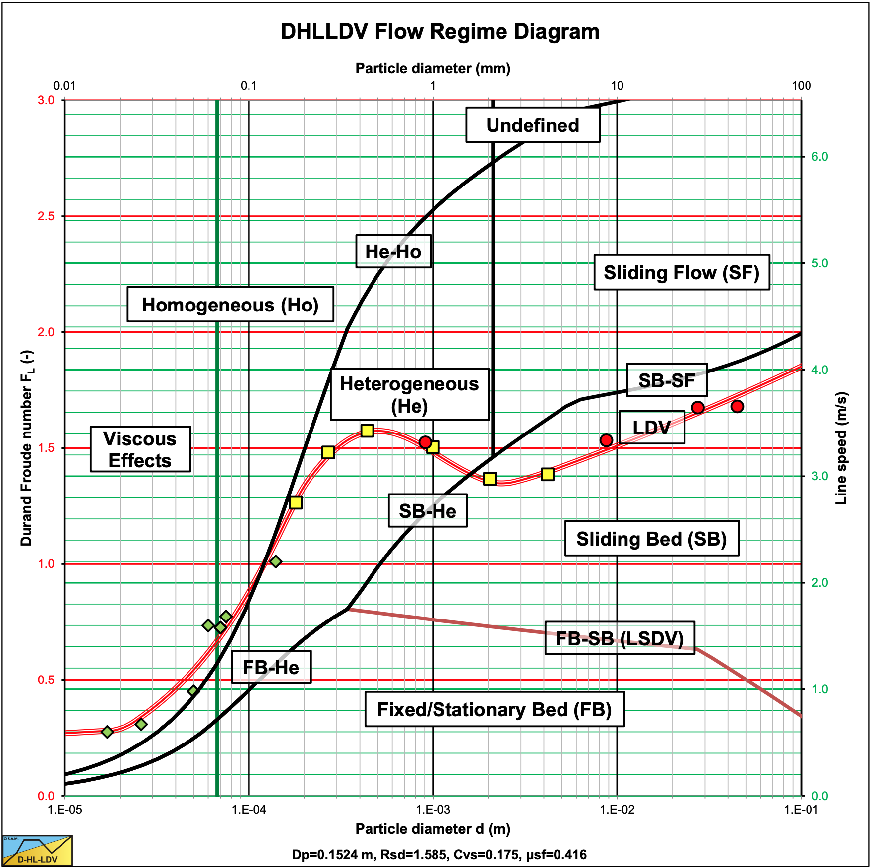
Figure 7.8-7 shows a resulting flow regime diagram, based on the transition velocities and the LDV. The transition curves are based on behavior. For example the transition SB-He shows when the flow transits from sliding bed behavior to heterogeneous behavior. This does not mean that at the transition there is still a sliding bed, it means up to the transition the hydraulic gradient is sliding friction dominated. This is the reason why the LDV curve can be below or above the transition curve. The LDV and the LSDV curves however do mean there is a sharp transition. The figure also shows upper limit LDV data from different sources. The green diamonds are from the Poloski et al. (2010) research of very fine particles. The yellow squares from Durand & Condolios (1952) of fine sands to fine gravels. The red circles are from Yagi et al. (1972) of medium sands to coarse gravel.

7.8.11 The Resulting Limit Deposit Velocity Curves

Now that the 5 transition velocities and the Limit Deposit Velocity have been found, how to apply them?

In slurry transport applications like dredging, the slurry transport process is not steady state, but dynamical. At the entrance of the pipeline the volumetric concentration and the particle size distribution, PSD, will vary in time. Because of this the hydraulic gradient will vary, resulting in a varying line speed. Even with steady state volumetric concentration and PSD, moving dunes and large vortices may occur. So to be safe, the maximum LDV curve should be used, which occurs at a volumetric concentration of about 20%.

Figure 7.8-8: The construction of the LDV curve.

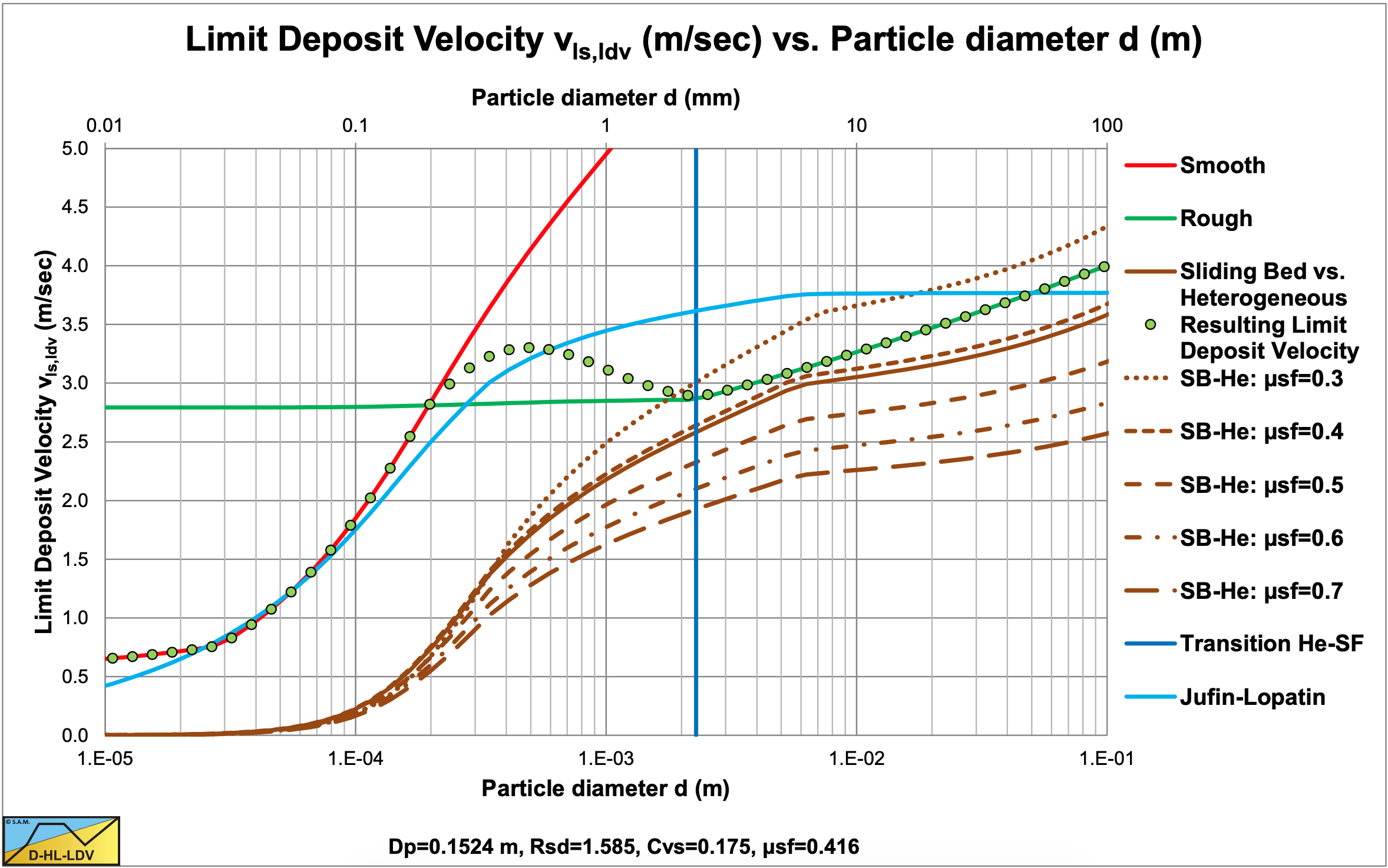
Figure 7.8-8 shows the construction of the LDV curve for sands and gravels in a 6 inch (0.1524 m) pipe, for a 20% volumetric concentration. Up to a particle diameter of about 0.15 mm the resulting curve follows the smooth curve (red line). From 0.15 mm to about 2 mm the resulting curve follows the transition equation. Above 2mm, in this case the transition velocity between the sliding bed regime and the heterogeneous regime is followed. Finally above about 10 mm the sliding flow criteria is followed. The shape of the curve depends strongly on the pipe diameter. With small diameter pipes, the transition velocity between the sliding bed regime and the heterogeneous regime will be dominant for larger particles. While for large pipe diameters as used in dredging, this will hardly have any influence. The graph also contains the Jufin & Lopatin (1966) LDV curve, which is a one equation curve. This equation is chosen because of the range of pipe diameters, from about 1 inch to 90 cm, investigated. Of course a one equation model can never result in a complex curve based on different criteria as is shown here. However for practical purposes it also gives a good and safe result.

Figure 7.8-9 shows the same LDV curve, but now with experimental data and as the Durand & Condolios LDV Froude number F_L. Each column of data points represents a series of experiments with different volumetric concentrations. The lowest points a concentration of 1-5%, the highest point a concentration of 15-25%.
Most of the data points above the curve are from pipe diameters smaller than 6 inch (0.1524 m). From these experiments it is concluded that the F_L value increases slightly with decreasing pipe diameter. The highest points are from the smallest pipe diameters. The Fuhrboter (1961) experiments were carried out in a 30 cm diameter pipe and it is clear that these points are lower.

Figure 7.8-9: The resulting LDV curve versus experimental data.

Figure 7.8-10: The resulting LDV curve for different concentrations on a linear axis.

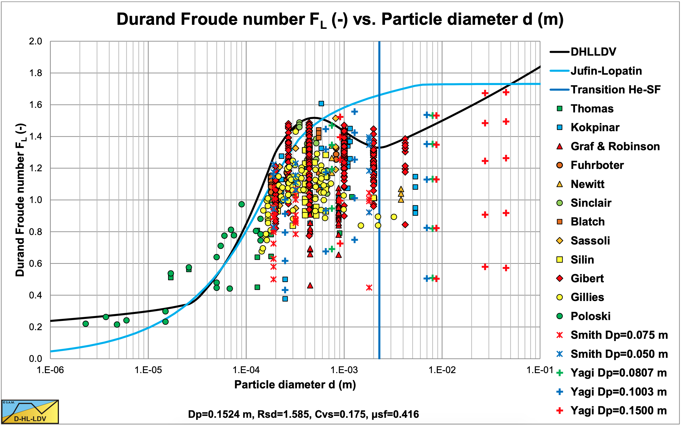
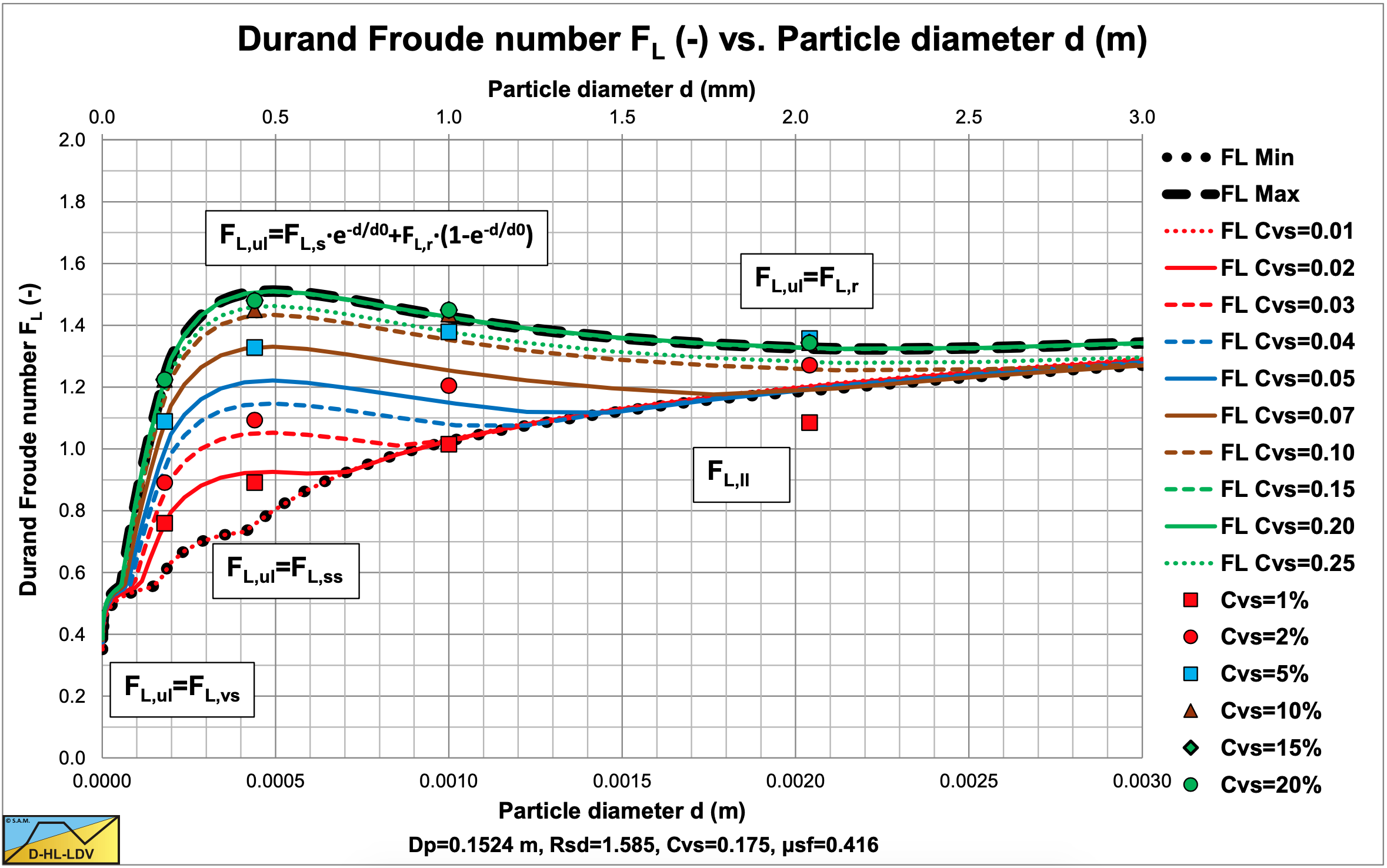
Figure 7.8-10 shows the resulting LDV curves for volumetric concentrations from 1% to 25% on a linear horizontal axis. The horizontal axis is limited to particles of 2.5 mm in order to compare this graph with the famous Durand & Condolios (1952) graph. Although the Durand & Condolios graph as copied by many authors contains an error on the vertical axis by a factor 1.285, giving an asymptotic value of 1.34 for large particles (which should have been 1.05), the resemblance with their graph is remarkable. Based on the experiments published by Gibert (1960) and others, the wrong Durand & Condolios graph seems to be the right graph. It is remarkable however that 1.285² equals 1.65, the relative submerged density of the quarts. It seems that in the original Durand & Condolios (1952) graph the relative submerged density was already taken into account, although not mentioned in their equation. A simple example may show this. The LDV’s measured were between 2.95 and 3.2 m/s in a 0.1524 m pipe. This gives an F_L value between 1.35 and 1.47 matching their latest graph very well.

Figure 7.8-11: The construction of the LDV curve for large diameter pipes.

Figure 7.8-12: The resulting LDV curve for different concentrations on a linear axis.

Figure 7.8-13: The construction of the LDV curve for a 30 cm diameter pipe.

Figure 7.8-14: The 30 cm pipe diameter LDV curve versus experimental data.

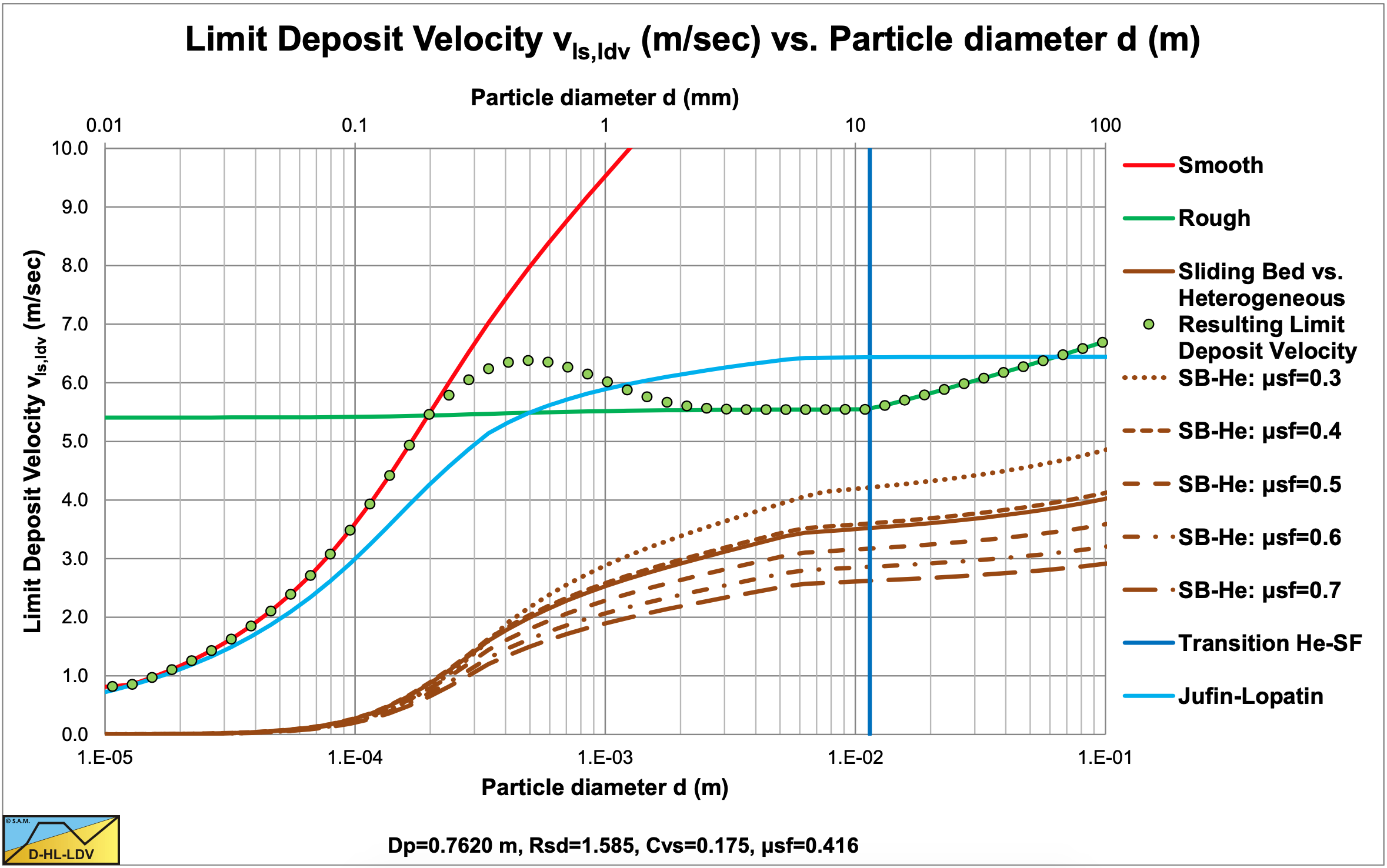
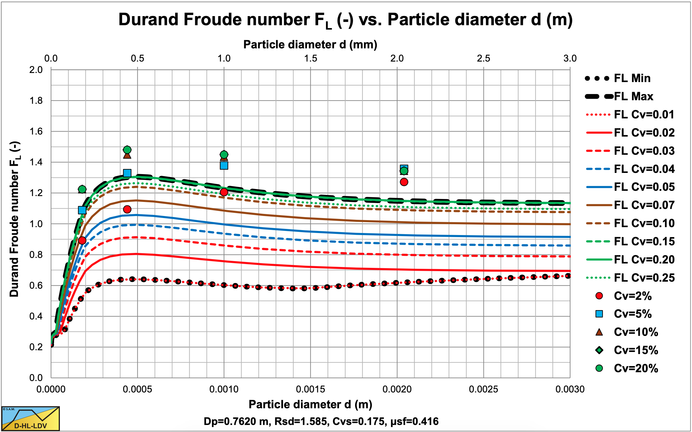
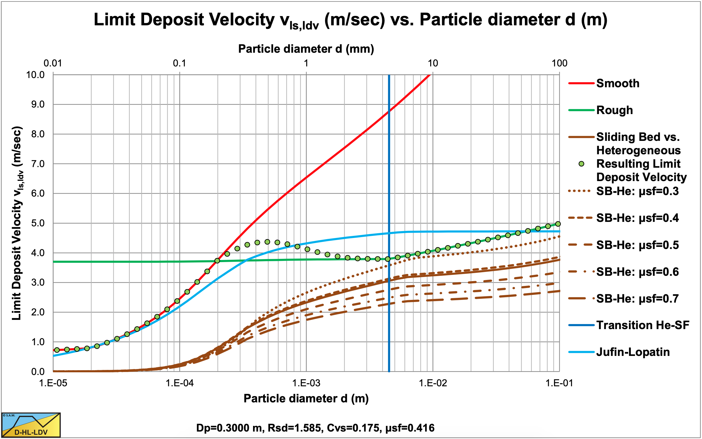
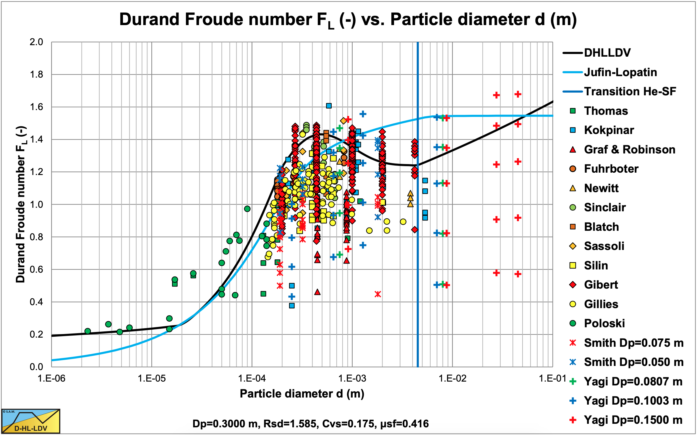
Figure 7.8-11 shows the construction of the LDV curve for large diameter pipes. For a volumetric concentration of about 20%, the transition velocity between the sliding bed and the heterogeneous regime does not play a role anymore. However at small concentrations it still does as is shown in Figure 7.8-12. The Jufin & Lopatin equation still matches well, although it underestimates the LDV for medium sands compared with the model developed here. It should be noted that the intersection point between a smooth and a rough bed is at a particle diameter of about 0.14 mm for all pipe diameters with sands and gravels. Figure 7.8-12 also shows that for large diameter pipes, the curves do not converge for larger particles, but each volumetric concentration has an LDV curve, unless the transition velocity between the sliding bed and the heterogeneous regime takes over.

Figure 7.8-13 and Figure 7.8-14 show the LDV curve for a 30 cm pipe and 20% volumetric concentration. The data points of Fuhrboter (1961) match the LDV curve closely.

It should be mentioned that not all researchers use the same methodology to determine the LDV. Yagi et al. (1972) determined the minimum hydraulic gradient velocity instead of the LDV. For high concentrations these are almost equal, but for low concentrations the minimum hydraulic gradient velocity is much smaller than the LDV, explaining the location of the data points at low concentrations.

Figure 7.8-15: The path of the LDV curve in a Erhg graph for a 6 inch (0.1524 m) pipe.

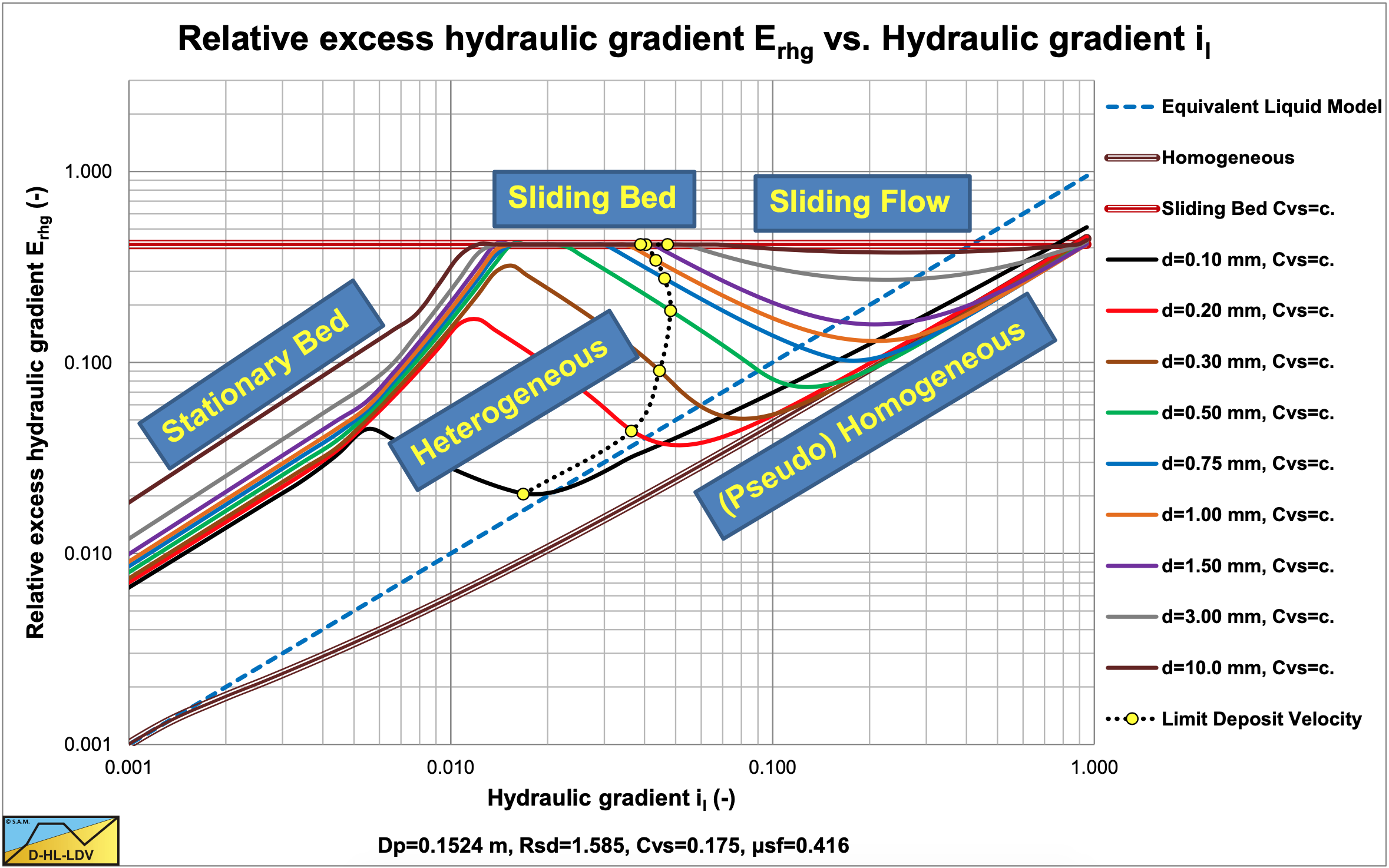
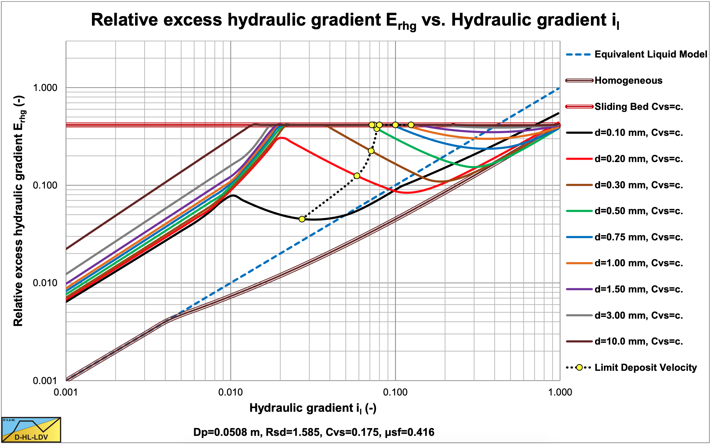
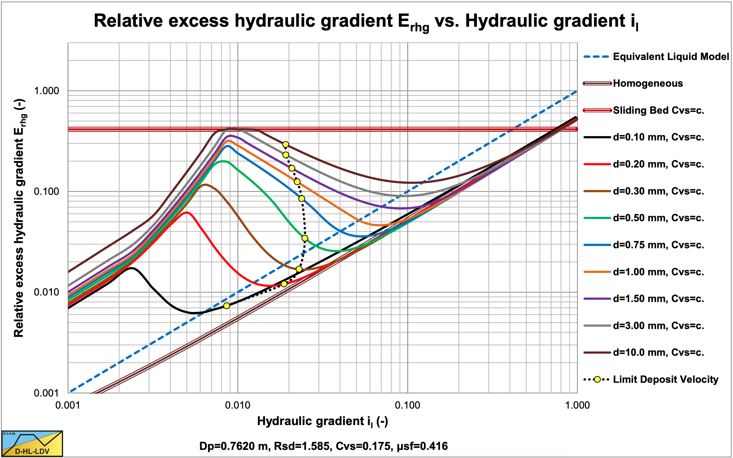
Figure 7.8-15 shows the path of the LDV curve in a E_rhg graph. The points are calculated for particle diameters of 0.1, 0.2, 0.3, 0.5, 0.75, 1, 1.5, 3 and 10 mm. It is shown that for very small particles the LDV follows the homogeneous curve closely. From 0.2 to 3 mm the curve transits from the homogeneous curve to the sliding bed curve. Above 3mm the LDV will follow the sliding bed curve. For smaller pipe diameters (Figure 7.8-16) the LDV curve moves to the right, meaning that the distance between the homogeneous curve and the sliding bed curve decreases. Particles smaller than 3 mm will already reach the sliding bed curve. For larger pipe diameters (Figure 7.8-17) the LDV curve moves to the left, meaning that the distance between the homogeneous curve and the sliding bed curve increases. Particles smaller than 3 mm will not even reach the sliding bed curve.

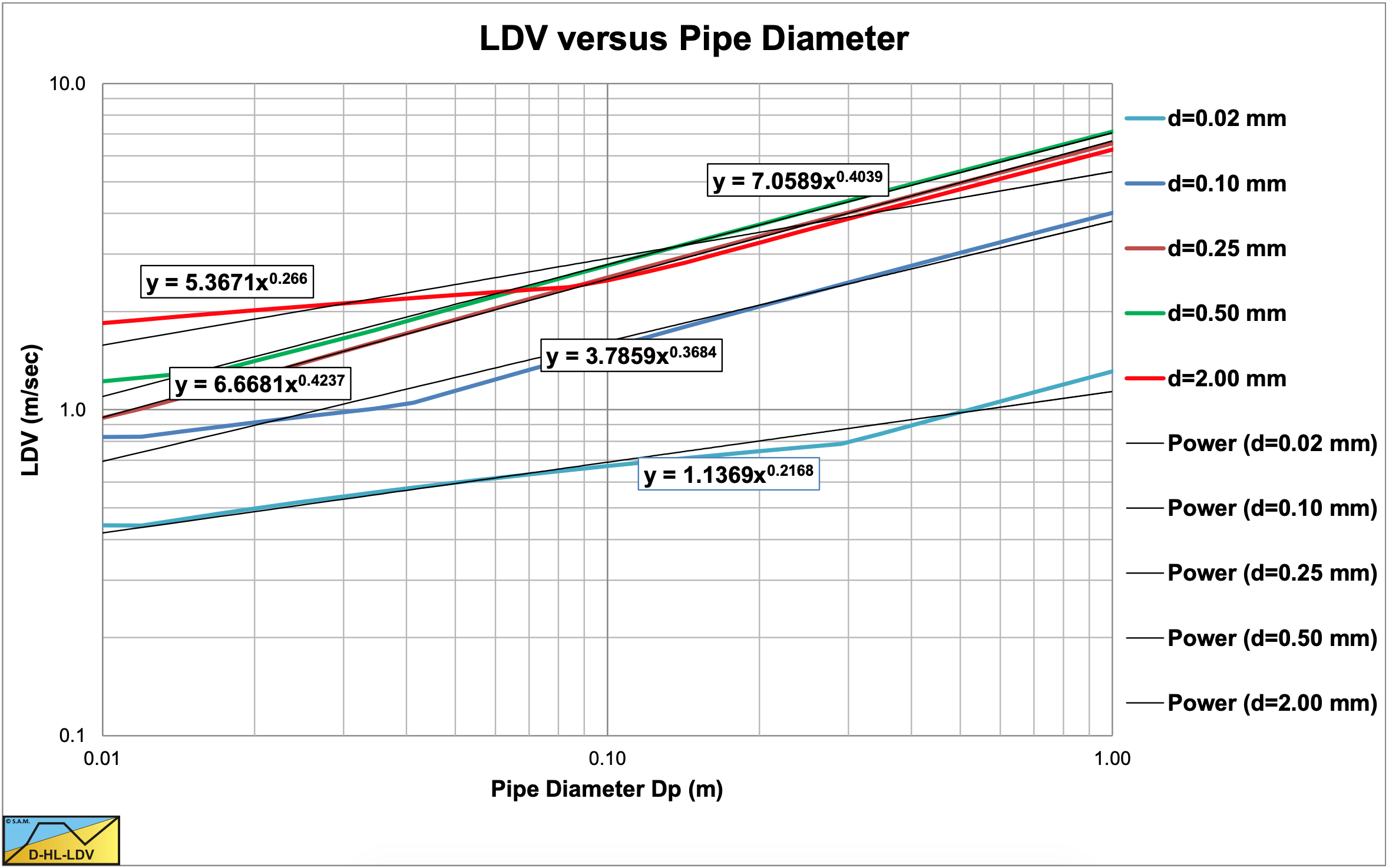
Figure 7.8-18 shows the LDV as a function of the pipe diameter for 5 different particle sizes. In the graph also the average powers of the LDV curves with respect to the pipe diameters are shown. Equations (7.8-37) and (7.8-51) give a power of 1/3 based on the presence of the pipe diameter in the equations. However, the equations also contain the Darcy-Weisbach friction factor in the denominator, increasing the powers slightly to a value around 0.4. For small diameter pipes, the limiting transition velocity between the sliding bed and the heterogeneous regime results in a flat part. For particles with d>0.015·D_p, the adjustment of the LDV according to equation (7.8-52) will reduce the power.

Based on this analysis, it is impossible to model the LDV with a one term equation. There are 5 different regions of the LDV and a limiting transition velocity. Very small particles, a smooth bed, a rough bed, a transition region and the criterion d>0.015·D_p together with the limiting transition velocity between the sliding bed and the heterogeneous regime. Curve fit techniques on experimental data will always give a result, but this will be a different result based on the particle and pipe diameters used in the experiments.

Figure 7.8-16: The path of the LDV curve in a E_rhg graph for a 2 inch (0.0508 m) pipe.

Figure 7.8-17: The path of the LDV curve in a E_rhg graph for a 30 inch (0.762 m) pipe.

Figure 7.8-18: The LDV as a function of the pipe diameter for 5 particle sizes.

Figure 7.8-19: The LDV as a function of the particle diameter for 5 pipe diameters.

7.8.12 Conclusions & Discussion

There are many definitions and names for the critical velocity. Here the critical velocity is defined as the Limit Deposit Velocity, the line speed above which there is no stationary bed or sliding bed. Below the LDV there may be either a stationary or fixed bed or a sliding bed, depending on the particle diameter and the pipe diameter and of course the liquid properties.

The DHLLDV Framework divides particles in 5 regions and a lower limit. These regions are for sand and gravel; very small particles up to about δ_v, small particles up to 0.2 mm, a transition region from 0.2 mm to 2 mm, particles larger than 2 mm and particles larger than 0.015 times the pipe diameter. The lower limit is the transition between a sliding bed and heterogeneous transport.

Each region is modelled separately, resulting in dynamic transition particle diameters, depending on the parameters involved. The modelling is independent of head loss models. The modelling is calibrated mainly with sand and gravel experimental data, although limited data is used for other relative submerged densities. The equations found give an upper limit to the LDV and are thus conservative, but safe.

Although the model seems completed, there are still a number of issues that required further investigation. For region 1, very fine particles, the liquid viscosity and density may need adjustment, however it is the question whether this is necessary in the viscous sub-layer. For region 5, very large particles, it is the question whether an LDV exists. At concentrations above a certain threshold (related to sheet flow) the bed concentration may decrease continuously. Still some characteristic LDV value is required to determine the slip velocity in the DHLLDV Framework. For all regions the relative submerged density has not yet been investigated thoroughly, although it is part of the model. For the limited data investigated the model gives good results, but more experimental data could adjust the implementation of the relative submerged density. For dredging purposes however the model is suitable.

In Figure 7.8-7 the flow regime transitions are determined based on the equations of each flow regime. This results in sharp flow regime transitions. In reality these transitions may be smooth. This is the reason why the LDV curve does not coincide exactly with the flow regime transitions.

7.8.13 Nomenclature Limit Deposit Velocity

Ap	Cross section pipe	m^2
AH	Cross section of the restricted area above the bed (also named A1)	m^2
Cvb	Bed volumetric concentration	-
Cvs	Spatial volumetric concentration	-
Cvs,ldv	Concentration of bed at LDV	-
Cvr,ldv	Bed fraction at LDV	-
Cvt	Transport or delivered volumetric concentration	-
Cx	Durand & Condolios coefficient	-
d	Particle diameter	m
d0	Transition particle diameter	m
Dp	Pipe diameter	m
DH	Hydraulic diameter cross section above the bed	m
Erhg	Relative excess hydraulic gradient	-
FL	Durand Limit Deposit Velocity Froude number	-
FL,s	Durand Limit Deposit Velocity Froude number smooth bed	-
FL,r	Durand Limit Deposit Velocity Froude number rough bed	-
Fsf	Sliding friction force	kN
FW	Weight of bed at LDV	kN
g	Gravitational constant (9.81)	m/s^2
h	Thickness of bed layer at LDV	m
il	Hydraulic gradient of liquid	-
im ​​​​​​​	Hydraulic gradient of mixture	-
im,sb	Hydraulic gradient sliding bed	-
isf	Hydraulic gradient solids effect sliding bed	-
im,fb	Hydraulic gradient fixed bed	-
im,ho	Hydraulic gradient homogeneous transport	-
is	Hydraulic gradient solids in homogeneous transport	-
ks	Bed roughness	m
ks^+	Dimensionless bed roughness	-
ΔL	Length of pipeline	m
n	Porosity of bed	-
Rsd	Relative submerged density	-
Re*	Roughness Reynolds number	-
u	Velocity above the bed	m/s
u*	Friction velocity	m/s
vls	Cross-section averaged line speed	m/s
vls,ldv	Line speed at Limit Deposit Velocity	m/s
vls,r	Line speed through restricted area above the bed	m/s
vls,sb-ho	Line speed at intersection sliding bed and homogeneous regimes	m/s
vt	Particle terminal settling velocity	m/s
y	Distance above the bed	m
y^+	Dimensionless distance above the bed	-
y0	Constant in logarithmic velocity profile	m
αp	Energy fraction coefficient	-
β	Richardson & Zaki hindered settling power	-
δv	Thickness of viscous sub layer	m
λl	Darcy-Weisbach friction factor between liquid and pipe wall	-
λr	Resulting Darcy Weisbach friction factor in restricted area above the bed	-
κ	Von Karman constant (about 0.4)	-
κC	Concentration eccentricity constant	-
ρl	Density of liquid	ton/m^3
νl	Kinematic viscosity liquid	m^2/s
μsf	Sliding friction coefficient	-
\(\ \tau_{12}\)	Bed shear stress	kPa
θ	Shields number	-