7.9: The Slip Velocity

7.9.1 Introduction

Miedema & Ramsdell (2013) derived a new model for determining the head losses in heterogeneous slurry transport based on energy considerations. The head losses consist of the viscous losses, potential energy losses and kinetic energy losses. The total pressure required to push the slurry mixture through the pipeline is:

\[\ \Delta \mathrm{p}_{\mathrm{m}}=\Delta \mathrm{p}_{\mathrm{l}}+\Delta \mathrm{p}_{\mathrm{s}, \mathrm{p o t}}+\Delta \mathrm{p}_{\mathrm{s}, \mathrm{k i n}}=\Delta \mathrm{p}_{\mathrm{l}} \cdot\left(\mathrm{1}+\dfrac{\Delta \mathrm{p}_{\mathrm{s}, \mathrm{p o t}}}{\Delta \mathrm{p}_{\mathrm{l}}}+\dfrac{\Delta \mathrm{p}_{\mathrm{s, kin}}}{\Delta \mathrm{p}_{\mathrm{l}}}\right)\]

This can also be written in terms of the hydraulic gradients according to:

\[\ \mathrm{i}_{\mathrm{m}}=\mathrm{i}_{\mathrm{l}}+\mathrm{i}_{\mathrm{s}, \mathrm{pot}}+\mathrm{i}_{\mathrm{s}, \mathrm{kin}}=\mathrm{i}_{\mathrm{l}} \cdot\left(1+\dfrac{\mathrm{i}_{\mathrm{s}, \mathrm{pot}}}{\mathrm{i}_{\mathrm{l}}}+\dfrac{\mathrm{i}_{\mathrm{s,kin}}}{\mathrm{i}_{\mathrm{l}}}\right)\]

The potential energy contribution to the excess head losses due to the solids effect can be written as:

\[\ \Delta \mathrm{p}_{\mathrm{s}, \mathrm{pot}}=\rho_{\mathrm{l}} \cdot\left(\dfrac{\mathrm{v}_{\mathrm{t}} \cdot\left(1-\dfrac{\mathrm{C}_{\mathrm{vs}}}{\kappa_{\mathrm{C}}}\right)^{\beta}}{\mathrm{v}_{\mathrm{ls}}}\right) \cdot \mathrm{g} \cdot \mathrm{R}_{\mathrm{sd}} \cdot \mathrm{C}_{\mathrm{vs}} \cdot \Delta \mathrm{L} \quad\text{ or }\quad \mathrm{i}_{\mathrm{s}, \mathrm{pot}}=\dfrac{\Delta \mathrm{p}_{\mathrm{s}, \mathrm{pot}}}{\rho_{\mathrm{l}} \cdot \mathrm{g} \cdot \Delta \mathrm{L}}=\left(\dfrac{\mathrm{v}_{\mathrm{t}} \cdot\left(1-\dfrac{\mathrm{C}_{\mathrm{vs}}}{\mathrm{\kappa}_{\mathrm{C}}}\right)^{\beta}}{\mathrm{v}_{\mathrm{ls}}}\right) \cdot \mathrm{R}_{\mathrm{sd}} \cdot \mathrm{C}_{\mathrm{vs}}\]

The kinetic energy contribution to the excess head losses due to the solids effect can be written as:

\[\ \Delta \mathrm{p}_{\mathrm{s}, \mathrm{k i n}}=\rho_{1} \cdot\left(\dfrac{\mathrm{v}_{\mathrm{sl}} }{\mathrm{v}_{\mathrm{t}}}\right)^{\mathrm{2}} \cdot \mathrm{g} \cdot \mathrm{R}_{\mathrm{s d}} \cdot \mathrm{C}_{\mathrm{v s}} \cdot \Delta \mathrm{L} \quad\text{ or }\quad \mathrm{i}_{\mathrm{s}, \mathrm{k i n}}=\dfrac{\Delta \mathrm{p}_{\mathrm{s}, \mathrm{k i n}}}{\rho_{\mathrm{l}} \cdot \mathrm{g} \cdot \Delta \mathrm{L}}=\left(\dfrac{\mathrm{v}_{\mathrm{sl}}}{\mathrm{v}_{\mathrm{t}}}\right)^{2} \cdot \mathrm{R}_{\mathrm{sd}} \cdot \mathrm{C}_{\mathrm{v} \mathrm{s}}\]

Giving for the total hydraulic gradient for head losses of a mixture in slurry transport:

\[\ \mathrm{i}_{\mathrm{m}}=\mathrm{i}_{\mathrm{l}} \cdot\left(\mathrm{1}+\dfrac{\left(\mathrm{2} \cdot \mathrm{g} \cdot \mathrm{R}_{\mathrm{s} \mathrm{d}} \cdot \mathrm{D}_{\mathrm{p}}\right)}{\lambda_{\mathrm{l}}} \cdot \mathrm{C}_{\mathrm{v} \mathrm{s}} \cdot \dfrac{\mathrm{1}}{\mathrm{v}_{\mathrm{l} \mathrm{s}}^{2}} \cdot\left(\mathrm{v}_{\mathrm{t}} \cdot\left(\mathrm{1}-\dfrac{\mathrm{C}_{\mathrm{v} \mathrm{s}}}{\mathrm{\kappa}_{\mathrm{C}}}\right)^{\beta} \cdot \dfrac{\mathrm{1}}{\mathrm{v}_{\mathrm{ls}}}+\left(\dfrac{\mathrm{v}_{\mathrm{sl}}}{\mathrm{v}_{\mathrm{t}}}\right)^{2}\right)\right)\]

For determining the viscous losses, the well-known Darcy Weisbach equation will be used:

\[\ \Delta \mathrm{p}_{\mathrm{l}}=\lambda_{\mathrm{l}}\left(\mathrm{R} \mathrm{e}_{\mathrm{fl}}\right) \cdot \dfrac{\Delta \mathrm{L}}{\mathrm{D}_{\mathrm{p}}} \cdot \dfrac{\mathrm{1}}{2} \cdot \rho_{\mathrm{l}} \cdot \mathrm{v}_{\mathrm{l s}}^{2} \quad\text{ or }\quad \mathrm{i}_{\mathrm{l}}=\dfrac{\Delta \mathrm{p}_{\mathrm{l}}}{\rho_{\mathrm{l}} \cdot \mathrm{g} \cdot \Delta \mathrm{L}}=\dfrac{\lambda_{\mathrm{l}}\left(\mathrm{R} \mathrm{e}_{\mathrm{fl}}\right) \cdot \mathrm{v}_{\mathrm{ls}}^{2}}{\mathrm{2} \cdot \mathrm{g} \cdot \mathrm{D}_{\mathrm{p}}}\]

The potential energy contribution, as already derived by Newitt et al. (1955), to the excess head losses depends on the terminal settling velocity v_t and on the hindered settling power β as determined by Richardson and Zaki (1954).

An equation for the transitional region (in m and m/sec) for v_t has been derived by Ruby & Zanke (1977):

\[\ \mathrm{v_{t}}=\dfrac{10 \cdot v_{\mathrm{l}}}{\mathrm{d}} \cdot \left(\sqrt{1+\dfrac{\mathrm{R_{s d} \cdot g \cdot d^{3}}}{100 \cdot v_{\mathrm{l}}^{2}}}-1\right)\]

This equation also gives good results for very fine and very large particles and has been used everywhere in this book developing the head loss model. According to Rowe (1987) the power β can be approximated by:

\[\ \beta=\dfrac{4.7+0.41 \cdot \operatorname{Re}_{\mathrm{p}}^{0.75}}{1+0.175 \cdot \operatorname{Re}_{\mathrm{p}}^{0.75}}\]

The kinetic energy contribution to the excess head losses depends on the ratio of the so called slip velocity v_sl to the line speed v_ls. For a derivation of equation (7.9-4), see Miedema &Ramsdell (2013). The slip velocity v_sl is defined as the difference between the average liquid velocity v_l and the average particle velocity v_p resulting in a drag force.

\[\ \mathrm{v}_{\mathrm{s l}}=\mathrm{v _ { l }}-\mathrm{v}_{\mathrm{p}}\]

This slip velocity v_sl however is unknown and not much has been published about this. This slip velocity however is very important for dredging practice and slurry transport in general because it determines the ratio of the so called volumetric transport (delivered) concentration C_vt to the volumetric spatial concentration C_vs. The spatial volumetric concentration C_vs is defined as the volume of solids divided by the volume of the mixture containing these solids. So the spatial volumetric concentration is based on a volume ratio, while the delivered volumetric concentration is based on a volume rate ratio. One of the few publications regarding the slip velocity is Yagi et al. (1972) who measured both concentrations in order to determine the slip velocity to line speed ratio.

7.9.2 Slip Ratio in the Heterogeneous Regime

Based on the analysis, the following coefficients (powers) are determined, not by mathematical regression, but by visual observation of graphs (Miedema (2014W)) of the experimental data. The reason for this is that very often the data points are in a transition region between two regimes and do not exactly follow the formulation of one of the regimes. Mathematical regression would lead to the wrong conclusions. Based on the new dimensionless parameters the following is found (the two formulations are based on the line speed ls or the friction velocity fv):

\[\ \begin{array}{left} \mathrm{v}_{\mathrm{s l}}=\frac{\mathrm{8.5}}{\sqrt{\lambda_{\mathrm{l}}}} \cdot \mathrm{C t} \cdot \mathrm{T h}_{\mathrm{ls}} \cdot \mathrm{v}_{\mathrm{t}}=\frac{\mathrm{8 . 5}}{\sqrt{\mathrm{8}}} \cdot \mathrm{C t} \cdot \mathrm{T h}_{\mathrm{f v}} \cdot \mathrm{v}_{\mathrm{t}}\\
\left(\frac{\mathrm{v}_{\mathrm{sl}}}{\mathrm{v}_{\mathrm{t}}}\right)^{2}=\frac{\mathrm{8 . 5}^{2}}{\lambda_{\mathrm{l}}} \cdot \mathrm{C t}^{2} \cdot \mathrm{Th}_{\mathrm{l s}}^{2}=\frac{\mathrm{8.5}^{2}}{\mathrm{8}} \cdot \mathrm{C t}^{2} \cdot \mathrm{T h}_{\mathrm{fv}}^{2} \end{array}\]

Substituting equation (7.9-10) in equation (7.9-5) gives for the hydraulic gradient:

\[\ \begin{array}{\left} \mathrm{i}_{\mathrm{m}}=\mathrm{i}_{\mathrm{l}} \cdot\left(1+\frac{\left(2 \cdot \mathrm{g} \cdot \mathrm{R}_{\mathrm{sd}} \cdot \mathrm{D}_{\mathrm{p}}\right)}{\lambda_{\mathrm{l}}} \cdot \mathrm{C}_{\mathrm{vs}} \cdot \frac{1}{\mathrm{v}_{\mathrm{ls}}^{2}} \cdot\left(\mathrm{L a}+\frac{8.5^{2}}{8} \cdot \mathrm{Ct}^{2} \cdot \mathrm{Th}_{\mathrm{fv}}^{2}\right)\right)\\
\text{or}\\
\mathrm{i}_{\mathrm{m}}=\mathrm{i}_{\mathrm{l}}+\left(\mathrm{L a}+\frac{\mathrm{8 . 5}^{2}}{\mathrm{8}} \cdot \mathrm{C t}^{2} \cdot \mathrm{Th}_{\mathrm{fv}}^{2}\right) \cdot \mathrm{R}_{\mathrm{sd}} \cdot \mathrm{C}_{\mathrm{vs}}\end{array}\]

The contribution of the kinetic energy losses to the excess head losses is completely determined by the two dimensionless numbers, Cát and Thủy (collision impact and collision intensity). The contribution of the potential energy losses to the excess head losses is completely determined by the ratio of the hindered terminal settling velocity to the line speed (the capability to form sediment), the dimensionless number Lắng (sedimentation capability). It is obvious from this analysis that the excess pressure losses should not be described by two Froude numbers, but by the collision impact number Ct (which is a Froude number), the collision intensity number Th and the sedimentation capability number La. It is also obvious that there is not just one term describing the excess head losses, but there are two terms, the first term describing the potential energy losses (the capability to form sediment) and a second term describing the kinetic energy losses (the collision impact influence times the collision intensity influence).

The time averaged slip ratio will be about 50% of the slip velocity as used to determine the kinetic energy losses. The slip velocity or ratio here is the value determined to explain for the kinetic energy losses, so in fact it is a delta slip velocity. So it is the difference between the maximum and minimum slip velocity. The average slip velocity is undetermined. Now this average will not differ to much from the slip velocity found and it is proposed to take this as the slip velocity. In fact as will be shown later, this part of the slip velocity at high line speeds is not to important for converting spatial to delivered concentration. So the slip ratio is about:

\[\ \xi=\frac{\mathrm{v}_{\mathrm{s l}}}{\mathrm{v}_{\mathrm{l s}}}=\frac{\mathrm{8 . 5}}{\sqrt{\lambda_{\mathrm{l}}}} \cdot \mathrm{C t} \cdot \mathrm{T h}_{\mathrm{l s}} \cdot \frac{\mathrm{v}_{\mathrm{t}}}{\mathrm{v}_{\mathrm{l} \mathrm{s}}}=\frac{\mathrm{8 . 5}}{\sqrt{\mathrm{8}}} \cdot \mathrm{C t} \cdot \mathrm{T h}_{\mathrm{f v}} \cdot \frac{\mathrm{v}_{\mathrm{t}}}{\mathrm{v}_{\mathrm{l s}}}\]

7.9.3 Comparison with the Yagi et al. (1972) Data Step 1

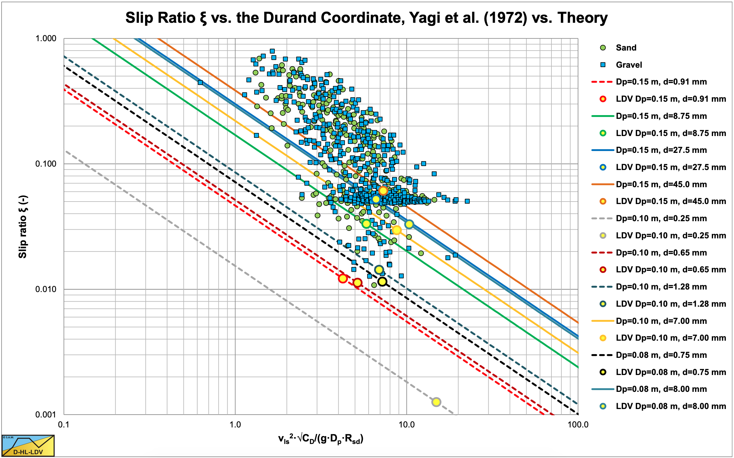
In order to validate the theoretical slip velocities, the data of Yagi et al. (1972) are available. Figure 7.9-1 shows the theoretical curves (equation (7.9-12)) for all the pipe diameter/particle diameter combinations Yagi et al. (1972) applied. It is remarkable that the theoretical curves for gravel (d=7 mm up to d=45 mm) match the data points pretty well, although they are a bit too low. In fact the theoretical lines are straight and miss the curvature required to match the data points better, however the Limit Deposit Velocities match on the horizontal axis but are too low. The theoretical curves for sand (d=0.25 mm up to d=1.28 mm) are all too low on the vertical axis. It should be mentioned that in the graph the theoretical curves are divided by 2, since the theoretical slip velocity equation determines the maximum slip velocity and not the time averaged slip velocity. Figure 7.9-1 shows that around the Limit Deposit Velocities the slip ratio should increase rapidly with a decreasing line speed, while at very low line speeds, the slip ratio should approach an asymptotic value, since the slip ratio can never be bigger than 1. Whether this asymptotic value is 1 or a value smaller than 1 is a question. If one considers that at a volumetric delivered concentration equal to the bed concentration, the slip ratio will be zero, since the whole bed is moving, an asymptotic slip ratio depending on the volumetric transport concentration is expected.

A second approach has to be considered for line speeds around and below the Limit Deposit Velocity.

Figure 7.9-1: The data of Yagi et al. (1972) compared with the theoretical slip velocities, step 1.

7.9.4 Derivation of the Slip Ratio at High A_b/A_p Ratios

When the A_b/A_p ratio is high, the slip ratio ξ might become larger than 1 according to Figure 7.9-1, which is physically impossible, so apparently the above equations are not valid for very low line speeds (around and below the Limit Deposit Velocity). In order to find a better estimate for the slip ratio in this case, the following logic is applied.

A fixed bed is considered, where it is assumed that the velocity above the bed is constant and equal to the line speed at the Limit Deposit Velocity. Further the constant transport concentration case is considered. The volumetric spatial concentration over the full cross section of the pipe can be related to the volumetric transport concentration over the full cross section of the pipe according to:

\[\ \mathrm{C}_{\mathrm{v s}}=\frac{\mathrm{A _ { b }} \cdot \mathrm{C}_{\mathrm{v b}}+\mathrm{A}_{\mathrm{s}} \cdot \mathrm{C}_{\mathrm{v s}, \mathrm{s}}}{\mathrm{A}_{\mathrm{p}}}=\left(\frac{\mathrm{v}_{\mathrm{l} \mathrm{s}}}{\mathrm{v}_{\mathrm{l} \mathrm{s}}-\mathrm{v}_{\mathrm{s l}}}\right) \cdot \mathrm{C}_{\mathrm{v} \mathrm{t}}\]

Suppose the volumetric spatial concentration C_vs,s and the volumetric transport concentration C_vt,s in the suspension phase are related according to their ratio at the transition velocity between the sliding bed regime or the fixed bed regime and the heterogeneous regime (the Limit Deposit Velocity):

\[\ \mathrm{C}_{\mathrm{v s}, \mathrm{s}}=\mathrm{\kappa}_{\mathrm{l d v}} \cdot \mathrm{C}_{\mathrm{v t}, \mathrm{s}}=\left(\frac{\mathrm{v}_{\mathrm{l s}, \mathrm{ld v}}}{\mathrm{v}_{\mathrm{l s}, \mathrm{l d v}}-\mathrm{v}_{\mathrm{s l}, \mathrm{l d} \mathrm{v}}}\right) \cdot \mathrm{C}_{\mathrm{v t}, \mathrm{s}} \quad\text{ with: }\quad \mathrm{\kappa}_{\mathrm{l d v}}=\left(\frac{\mathrm{v}_{\mathrm{l s}, \mathrm{ld v}}}{\mathrm{v}_{\mathrm{l s}, \mathrm{l d v}}-\mathrm{v}_{\mathrm{s l}, \mathrm{l d v}}}\right)=\left(\frac{\mathrm{1}}{\mathrm{1 - \xi _ { \mathrm { ldv } }}}\right)\]

Where κ_ldv equals the ratio between the two volumetric concentrations at the line speed v_ls,ldv where the sliding or fixed bed regime transits to the heterogeneous regime (LDV). Because there are only particles being transported in the suspension phase, the transport of particles over the full cross section has to be equal to the transport of particles in the suspension phase, thus:

\[\ \begin{array}{left} \mathrm{A}_{\mathrm{p}} \cdot \mathrm{C}_{\mathrm{v} \mathrm{t}} \cdot \mathrm{v}_{\mathrm{l} \mathrm{s}}=\mathrm{A}_{\mathrm{s}} \cdot \mathrm{C}_{\mathrm{v} \mathrm{t}, \mathrm{s}} \cdot \mathrm{v}_{\mathrm{s}}\\
\mathrm{W i t h}: \quad \mathrm{A}_{\mathrm{p}} \cdot \mathrm{v}_{\mathrm{l} \mathrm{s}}=\mathrm{A}_{\mathrm{s}} \cdot \mathrm{v}_{\mathrm{s}} \quad \Rightarrow \quad \mathrm{C}_{\mathrm{vt}}=\mathrm{C}_{\mathrm{v} \mathrm{t}, \mathrm{s}}\end{array}\]

This implies that the volumetric transport concentration over the full cross section of the pipe equals the volumetric transport concentration in the suspension phase. The volumetric spatial concentration in the suspension phase is assumed to be constant when there is a fixed bed/sliding bed below the LDV and can be written as:

\[\ \mathrm{C}_{\mathrm{v s}, \mathrm{s}}=\mathrm{\kappa}_{\mathrm{l} \mathrm{d} \mathrm{v}} \cdot \mathrm{C}_{\mathrm{v} \mathrm{t}}\]

The volumetric spatial concentration over the full cross section of the pipe can now be written as:

\[\ \mathrm{C}_{\mathrm{v s}}=\frac{\mathrm{A}_{\mathrm{b}} \cdot \mathrm{C}_{\mathrm{v b}}+\mathrm{A}_{\mathrm{s}} \cdot \mathrm{C}_{\mathrm{v s}, \mathrm{s}}}{\mathrm{A}_{\mathrm{p}}}=\frac{\mathrm{A}_{\mathrm{b}} \cdot \mathrm{C}_{\mathrm{v} \mathrm{b}}+\mathrm{A}_{\mathrm{s}} \cdot \mathrm{\kappa}_{\mathrm{l} \mathrm{d} \mathrm{v}} \cdot \mathrm{C}_{\mathrm{v} \mathrm{t}}}{\mathrm{A}_{\mathrm{p}}}=\left(\frac{\mathrm{v}_{\mathrm{l} \mathrm{s}}}{\mathrm{v}_{\mathrm{l} \mathrm{s}}-\mathrm{v}_{\mathrm{s} \mathrm{l}}}\right) \cdot \mathrm{C}_{\mathrm{v} \mathrm{t}}\]

The line speed and slip velocity in this equation are both related to the full cross section of the pipe. The cross section of the suspension phase equals the full cross section of the pipe minus the cross section of the fixed bed/sliding bed.

\[\ \mathrm{A}_{\mathrm{p}} \cdot \mathrm{C}_{\mathrm{v s}}=\mathrm{A}_{\mathrm{b}} \cdot \mathrm{C}_{\mathrm{v b}}+\left(\mathrm{A}_{\mathrm{p}}-\mathrm{A}_{\mathrm{b}}\right) \cdot \mathrm{\kappa}_{\mathrm{l d v}} \cdot \mathrm{C}_{\mathrm{v t}}=\mathrm{A}_{\mathrm{p}} \cdot\left(\frac{\mathrm{v}_{\mathrm{l s}}}{\mathrm{v}_{\mathrm{l s}}-\mathrm{v}_{\mathrm{s l}}}\right) \cdot \mathrm{C}_{\mathrm{v t}}\]

Separating the terms with the bed cross section and the pipe cross section gives:

\[\ \mathrm{A}_{\mathrm{b}} \cdot\left(\mathrm{C}_{\mathrm{v b}}-\mathrm{\kappa}_{\mathrm{l d v}} \cdot \mathrm{C}_{\mathrm{v t}}\right)+\mathrm{A}_{\mathrm{p}} \cdot \mathrm{\kappa}_{\mathrm{l d v}} \cdot \mathrm{C}_{\mathrm{v t}}=\mathrm{A}_{\mathrm{p}} \cdot\left(\frac{\mathrm{v}_{\mathrm{l s}}}{\mathrm{v}_{\mathrm{l s}}-\mathrm{v}_{\mathrm{s l}}}\right) \cdot \mathrm{C}_{\mathrm{v t}}\]

Or:

\[\ \mathrm{A}_{\mathrm{b}} \cdot\left(\mathrm{C}_{\mathrm{v b}}-\mathrm{\kappa}_{\mathrm{l d v}} \cdot \mathrm{C}_{\mathrm{v t}}\right) \cdot\left(\mathrm{v}_{\mathrm{l s}}-\mathrm{v}_{\mathrm{s l}}\right)+\mathrm{A}_{\mathrm{p}} \cdot \mathrm{\kappa}_{\mathrm{l d v}} \cdot \mathrm{C}_{\mathrm{v t}} \cdot\left(\mathrm{v}_{\mathrm{l s}}-\mathrm{v}_{\mathrm{s l}}\right)=\mathrm{A}_{\mathrm{p}} \cdot \mathrm{C}_{\mathrm{v t}} \cdot \mathrm{v}_{\mathrm{l} \mathrm{s}}\]

To find the slip ratio ξ, all the terms with the slip velocity have to be separated from the terms with the line speed according to:

\[\ \begin{array}{left} \mathrm{A}_{\mathrm{b}} \cdot\left(\mathrm{C}_{\mathrm{v} \mathrm{b}}-\mathrm{\kappa}_{\mathrm{l} \mathrm{d v}} \cdot \mathrm{C}_{\mathrm{v} \mathrm{t}}\right) \cdot \mathrm{v}_{\mathrm{l} \mathrm{s}}-\mathrm{A}_{\mathrm{b}} \cdot\left(\mathrm{C}_{\mathrm{v} \mathrm{b}}-\mathrm{\kappa}_{\mathrm{l} \mathrm{d v}} \cdot \mathrm{C}_{\mathrm{v t}}\right) \cdot \mathrm{v}_{\mathrm{s l}}+\mathrm{A}_{\mathrm{p}} \cdot \mathrm{\kappa}_{\mathrm{l d v}} \cdot \mathrm{C}_{\mathrm{v} \mathrm{t}} \cdot \mathrm{v}_{\mathrm{l s}}-\mathrm{A}_{\mathrm{p}} \cdot \mathrm{\kappa}_{\mathrm{l d v}} \cdot \mathrm{C}_{\mathrm{v t}} \cdot \mathrm{v}_{\mathrm{sl}}
=\mathrm{A}_{\mathrm{p}} \cdot \mathrm{C}_{\mathrm{v t}} \cdot \mathrm{v}_{\mathrm{l} \mathrm{s}}\\
\left(\mathrm{A}_{\mathrm{b}} \cdot\left(\mathrm{C}_{\mathrm{v b}}-\mathrm{\kappa}_{\mathrm{l d v}} \cdot \mathrm{C}_{\mathrm{v t}}\right)+\mathrm{A}_{\mathrm{p}} \cdot \mathrm{\kappa}_{\mathrm{l d v}} \cdot \mathrm{C}_{\mathrm{v t}}\right) \cdot \mathrm{v}_{\mathrm{l s}}-\left(\mathrm{A}_{\mathrm{b}} \cdot\left(\mathrm{C}_{\mathrm{v b}}-\mathrm{\kappa}_{\mathrm{l d v}} \cdot \mathrm{C}_{\mathrm{v t}}\right)+\mathrm{A}_{\mathrm{p}} \cdot \mathrm{\kappa}_{\mathrm{l d v}} \cdot \mathrm{C}_{\mathrm{v t}}\right) \cdot \mathrm{v}_{\mathrm{s l}}=\mathrm{A}_{\mathrm{p}} \cdot \mathrm{C}_{\mathrm{v t}} \cdot \mathrm{v}_{\mathrm{l s}}\end{array}\]

Giving:

\[\ \begin{array}{left}\xi=\frac{\mathrm{v}_{\mathrm{s l}}}{\mathrm{v}_{\mathrm{l s}}}=\frac{\mathrm{A}_{\mathrm{b}} \cdot\left(\mathrm{C}_{\mathrm{v b}}-\mathrm{\kappa}_{\mathrm{l d v}} \cdot \mathrm{C}_{\mathrm{v t}}\right)+\mathrm{A}_{\mathrm{p}} \cdot \mathrm{\kappa}_{\mathrm{l d v}} \cdot \mathrm{C}_{\mathrm{v t}}-\mathrm{A}_{\mathrm{p}} \cdot \mathrm{C}_{\mathrm{v} \mathrm{t}}}{\mathrm{A}_{\mathrm{b}} \cdot\left(\mathrm{C}_{\mathrm{v b}}-\mathrm{\kappa}_{\mathrm{l d v}} \cdot \mathrm{C}_{\mathrm{v t}}\right)+\mathrm{A}_{\mathrm{p}} \cdot \mathrm{\kappa}_{\mathrm{ldv}} \cdot \mathrm{C}_{\mathrm{v t}}}\\
\text{With : }\quad \hat{\mathrm{A}}_{\mathrm{b}}=\frac{\mathrm{A}_{\mathrm{b}}}{\mathrm{A}_{\mathrm{p}}} \Rightarrow \xi=\frac{\mathrm{v}_{\mathrm{sl}}}{\mathrm{v}_{\mathrm{ls}}}=\frac{\hat{\mathrm{A}}_{\mathrm{b}} \cdot\left(\mathrm{C}_{\mathrm{v} \mathrm{b}}-\mathrm{\kappa}_{\mathrm{l} \mathrm{d} \mathrm{v}} \cdot \mathrm{C}_{\mathrm{v} \mathrm{t}}\right)+\left(\kappa_{\mathrm{l} \mathrm{d} \mathrm{v}}-\mathrm{1}\right) \cdot \mathrm{C}_{\mathrm{vt}}}{\hat{\mathrm{A}}_{\mathrm{b}} \cdot\left(\mathrm{C}_{\mathrm{v b}}-\mathrm{\kappa}_{\mathrm{l d v}} \cdot \mathrm{C}_{\mathrm{v} \mathrm{t}}\right)+\kappa_{\mathrm{ldv}} \cdot \mathrm{C}_{\mathrm{v t}}}\end{array}\]

And for the bed fraction:

\[\ \hat{\mathrm{A}}_{\mathrm{b}}=\frac{\mathrm{A}_{\mathrm{b}}}{\mathrm{A}_{\mathrm{p}}}=\frac{\mathrm{C}_{\mathrm{v t}} \cdot\left(\mathrm{v}_{\mathrm{l} \mathrm{s}} \cdot\left(\mathrm{1}-\mathrm{\kappa}_{\mathrm{l} \mathrm{d} \mathrm{v}}\right)+\mathrm{\kappa}_{\mathrm{l} \mathrm{d} \mathrm{v}} \cdot \mathrm{v}_{\mathrm{s} \mathrm{l}}\right)}{\left(\mathrm{C}_{\mathrm{v} \mathrm{b}}-\mathrm{\kappa}_{\mathrm{l d} \mathrm{v}} \cdot \mathrm{C}_{\mathrm{v t}}\right) \cdot\left(\mathrm{v}_{\mathrm{l s}}-\mathrm{v}_{\mathrm{s l}}\right)}\]

Based on the line speed of transition between the fixed bed regime and the heterogeneous regime and the mixture velocity in the suspension phase, the following is valid:

\[\ \begin{array}{left} \mathrm{A}_{\mathrm{p}} \cdot \mathrm{v}_{\mathrm{l} \mathrm{s}}=\mathrm{A}_{\mathrm{s}} \cdot \mathrm{v}_{\mathrm{s}, \mathrm{l d v}}=\left(\mathrm{A}_{\mathrm{p}}-\mathrm{A}_{\mathrm{b}}\right) \cdot \mathrm{v}_{\mathrm{s}, \mathrm{l d v}}\\
\mathrm{A}_{\mathrm{b}} \cdot \mathrm{v}_{\mathrm{s}, \mathrm{l d v}}=\mathrm{A}_{\mathrm{p}} \cdot\left(\mathrm{v}_{\mathrm{s}, \mathrm{l d v}}-\mathrm{v}_{\mathrm{l s}}\right) \quad \Rightarrow \quad \hat{\mathrm{A}}_{\mathrm{b}}=\frac{\mathrm{A}_{\mathrm{b}}}{\mathrm{A}_{\mathrm{p}}}=\frac{\mathrm{v}_{\mathrm{s}, \mathrm{l} \mathrm{d} \mathrm{v}}-\mathrm{v}_{\mathrm{ls}}}{\mathrm{v}_{\mathrm{s,ldv}}}\end{array}\]

This gives for the slip ratio ξ:

\[\ \xi=\frac{\mathrm{v}_{\mathrm{s} \mathrm{l}}}{\mathrm{v}_{\mathrm{l s}}}=\frac{\left(\frac{\mathrm{v}_{\mathrm{s}, \mathrm{l} \mathrm{d} \mathrm{v}}-\mathrm{v}_{\mathrm{l s}}}{\mathrm{v}_{\mathrm{s}, \mathrm{l d v}}}\right) \cdot\left(\mathrm{C}_{\mathrm{v b}}-\mathrm{\kappa}_{\mathrm{l d v}} \cdot \mathrm{C}_{\mathrm{v t}}\right)+\left(\mathrm{\kappa}_{\mathrm{l d v}}-\mathrm{1}\right) \cdot \mathrm{C}_{\mathrm{v t}}}{\left(\frac{\mathrm{v}_{\mathrm{s}, \mathrm{l d v}}-\mathrm{v}_{\mathrm{l s}}}{\mathrm{v}_{\mathrm{s}, \mathrm{l d v}}}\right) \cdot\left(\mathrm{C}_{\mathrm{v b}}-\mathrm{\kappa}_{\mathrm{l d v}} \cdot \mathrm{C}_{\mathrm{v t}}\right)+\mathrm{\kappa}_{\mathrm{l d v}} \cdot \mathrm{C}_{\mathrm{v t}}}\]

Rewriting this equation gives the following equation for the slip ratio ξ assuming a fixed bed below the LDV:

\[\ \xi=\frac{\mathrm{v}_{\mathrm{sl}}}{\mathrm{v}_{\mathrm{l s}}}=1-\frac{\mathrm{C}_{\mathrm{v t}}}{\left(\frac{\mathrm{v}_{\mathrm{s}, \mathrm{ld} \mathrm{v}}-\mathrm{v}_{\mathrm{l s}}}{\mathrm{v}_{\mathrm{s}, \mathrm{l} \mathrm{d} \mathrm{v}}}\right) \cdot\left(\mathrm{C}_{\mathrm{v} \mathrm{b}}-\mathrm{\kappa}_{\mathrm{l d v}} \cdot \mathrm{C}_{\mathrm{v t}}\right)+\mathrm{\kappa}_{\mathrm{l d v}} \cdot \mathrm{C}_{\mathrm{v t}}}\]

Because at the LDV the full cross section is suspension this can be written as:

\[\ \xi=\frac{\mathrm{v}_{\mathrm{s} \mathrm{l}}}{\mathrm{v}_{\mathrm{ls}}}=1-\frac{\mathrm{C}_{\mathrm{v} \mathrm{t}} \cdot \mathrm{v}_{\mathrm{l s}, \mathrm{ld} \mathrm{v}}}{\left(\mathrm{C}_{\mathrm{v b}}-\mathrm{\kappa}_{\mathrm{l d v}} \cdot \mathrm{C}_{\mathrm{v t}}\right) \cdot\left(\mathrm{v}_{\mathrm{l s}, \mathrm{l} \mathrm{d} \mathrm{v}}-\mathrm{v}_{\mathrm{l s}}\right)+\mathrm{\kappa}_{\mathrm{l d v}} \cdot \mathrm{C}_{\mathrm{v t}} \cdot \mathrm{v}_{\mathrm{l s}, \mathrm{l d v}}}\]

Case 1: The line speed vls equals the Limit Deposit Velocity v_ls,ldv=v_s,ldv:

\[\ \xi_{\mathrm{ldv}}=\frac{\mathrm{v}_{\mathrm{sl}}}{\mathrm{v}_{\mathrm{l s}}}=1-\frac{\mathrm{C}_{\mathrm{v t}} \cdot \mathrm{v}_{\mathrm{l s}, \mathrm{l d v}}}{\left(\mathrm{C}_{\mathrm{v b}}-\mathrm{\kappa}_{\mathrm{l d v}} \cdot \mathrm{C}_{\mathrm{v t}}\right) \cdot\left(\mathrm{v}_{\mathrm{l s}, \mathrm{ld v}}-\mathrm{v}_{\mathrm{l s}, \mathrm{l d v}}\right)+\mathrm{\kappa}_{\mathrm{l d v}} \cdot \mathrm{C}_{\mathrm{v t}} \cdot \mathrm{v}_{\mathrm{l s}, \mathrm{l d v}}}=\mathrm{1}-\frac{\mathrm{1}}{\mathrm{\kappa}_{\mathrm{l d v}}}=\frac{\mathrm{v}_{\mathrm{s l}, \mathrm{l d v}}}{\mathrm{v}_{\mathrm{l s}, \mathrm{l d v}}}\]

This is correct, since the factor κ_ldv was introduced as the ratio between the volumetric spatial concentration to the volumetric transport concentration at the LDV.

Case 2: the line speed v_ls equals zero:

\[\ \xi_{0}=\frac{\mathrm{v}_{\mathrm{sl}}}{\mathrm{v}_{\mathrm{ls}}}=1-\frac{\mathrm{C}_{\mathrm{v t}} \cdot \mathrm{v}_{\mathrm{l} \mathrm{s}, \mathrm{l} \mathrm{d} \mathrm{v}}}{\left(\mathrm{C}_{\mathrm{v} \mathrm{b}}-\mathrm{\kappa}_{\mathrm{l} \mathrm{d} \mathrm{v}} \cdot \mathrm{C}_{\mathrm{v t}}\right) \cdot\left(\mathrm{v}_{\mathrm{l} \mathrm{s}, \mathrm{ld} \mathrm{v}}-\mathrm{0}\right)+\mathrm{\kappa}_{\mathrm{l d v}} \cdot \mathrm{C}_{\mathrm{v} \mathrm{t}} \cdot \mathrm{v}_{\mathrm{l} \mathrm{s}, \mathrm{ld} \mathrm{v}}}=\mathrm{1}-\frac{\mathrm{C}_{\mathrm{v} \mathrm{t}}}{\mathrm{C}_{\mathrm{vb}}}\]

The slip ratio now depends on the volumetric transport concentration and is equal to 0 if the volumetric transport concentration is equal to the bed concentration, a bed moving with the line speed.

The assumption of having a fixed bed with a constant speed above the fixed bed is questionable. In reality there will be a sliding bed above a certain line speed, resulting in a different slip ratio at constant transport concentration. The equation as derived here can be considered to give an upper limit of the slip ratio.

7.9.5 Comparison with the Yagi et al. (1972) Data Step 2

Incorporating the upper limit for the slip velocity according equation (7.9-26) for line speeds below the Limit Deposit Velocity gives the result for very low concentrations (C_vt=0.05) as shown in Figure 7.9-2 and for the highest concentrations as used by Yagi et al. (1972) (C_vt=0.11-0.34) this is shown in Figure 7.9-3. Both figures also show the Limit Deposit Velocities for the different sands and gravels. The abscissa of the Limit Deposit Velocities is determined with the theory in chapter 7.8, the ordinate with equation (7.9-32).

Figure 7.9-2: The data of Yagi et al. (1972) compared with the theoretical slip velocities, step 2, C_vt=0.05.

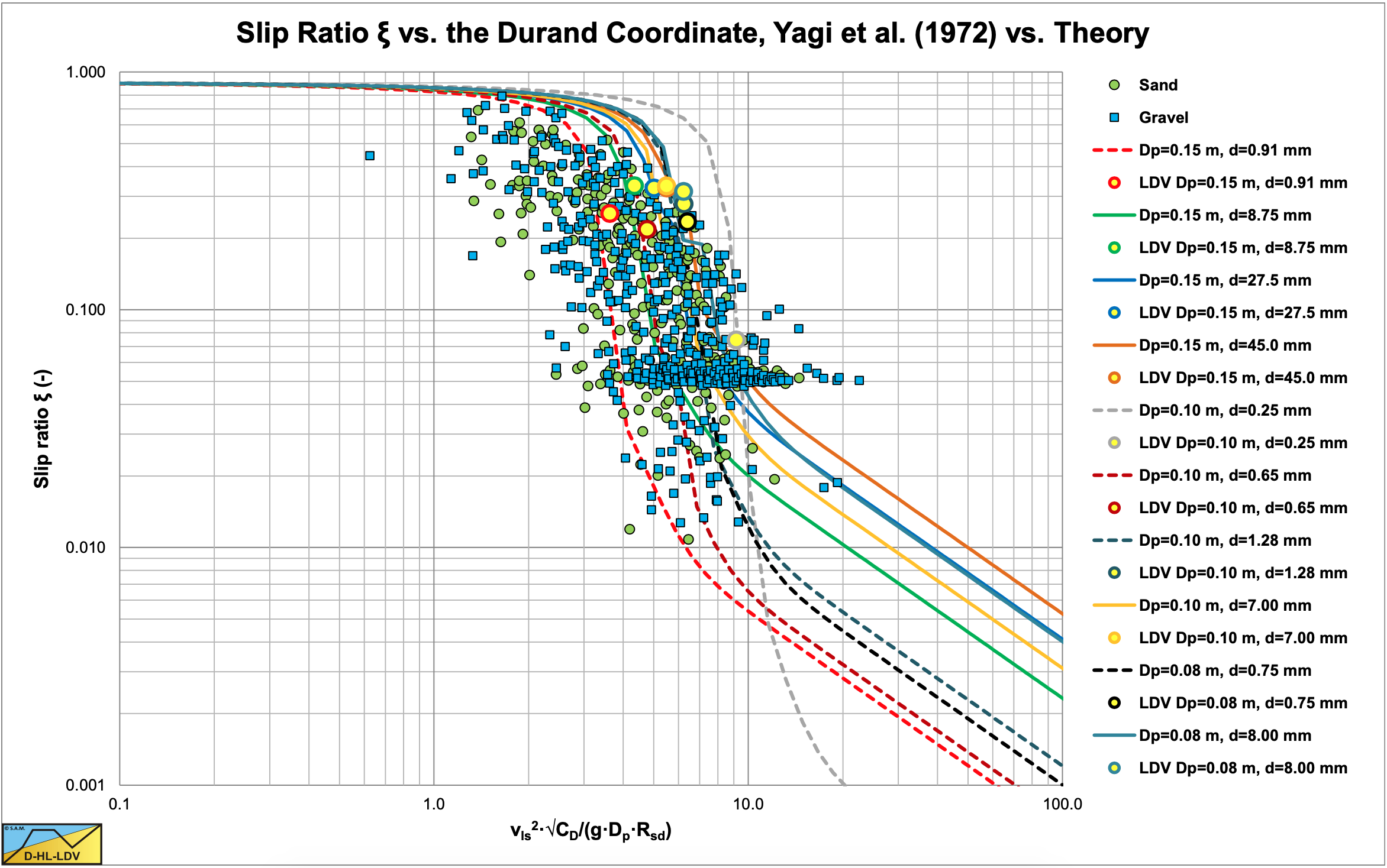
The original data of Yagi et al. (1972) show that the data points of sand and gravel overlap and that for each type of sand and gravel, data points are found on the left, on the right and in the middle of the cloud of points. At a slip ratio of 0.04-0.08 there is a concentration of data points both for sands and gravels. Since Yagi et al. (1972) carried out experiments below and above the Limit Deposit Velocity about 50/50, it is expected that the slip ratio at the Limit Deposit Velocity will be above this concentration of data points. How far above depends on the type of material and on the volumetric concentration of the experiments.

Figure 7.9-3: The data of Yagi et al. (1972) compared with the theoretical slip velocities, step 2, C_vt=0.11-0.34.

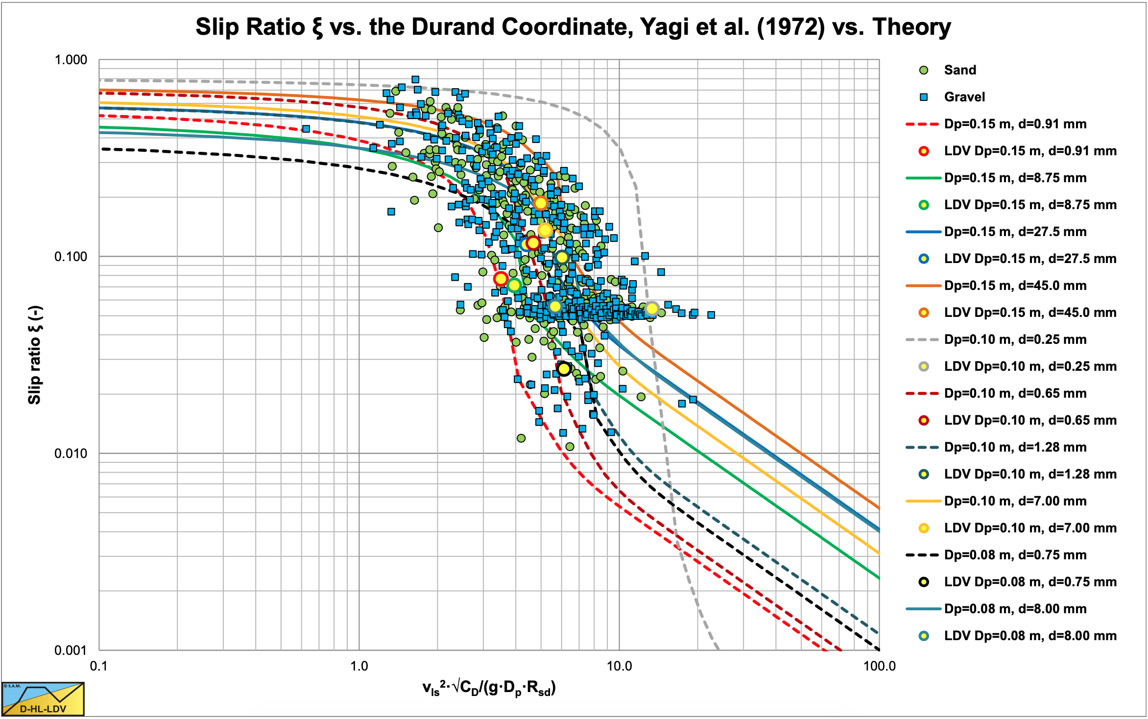
Figure 7.9-2 and Figure 7.9-3 show a sudden increase of the slip ratio with a decreasing line speed close to the Limit Deposit Velocity. Both graphs also show an asymptotic behavior at very low line speeds, matching the data points. With a minimum volumetric concentration of about 5% (Figure 7.9-2) and a maximum volumetric concentration from 11% to 34% depending on the material (Figure 7.9-3) the curvature of the data points is covered completely. Close to the Limit Deposit Velocity however, the slip ratio is overestimated. This is caused by the fact that equation (7.9-26) is based on a fixed bed and not on a sliding bed. Considering a fixed volumetric delivered concentration, a fixed bed approach will give a much higher slip ratio than a sliding bed approach, since the fact that the bed is sliding always reduces the slip ratio. Apparently there are 3 regions regarding the slip ratio. The region of line speeds much lower than the Limit Deposit Velocity, the region of line speeds around the Limit Deposit Velocity and the region of line speeds higher than the Limit Deposit Velocity. For the region around the Limit Deposit Velocity an approach has to be found.

7.9.6 The Region around the Limit Deposit Velocity

For very low line speeds, the slip ratio approaches (1-C_vt/C_vb) according to equation (7.9-27). For line speeds above the Limit Deposit Velocity, the slip ratio will behave according to equation (7.9-10) divided by 2, because this equation gives the maximum slip velocity and here the time averaged slip velocity is required. Yagi et al. (1972) found that the slip ratio decreases with the line speed to a power of -2.8, based on their measurements.

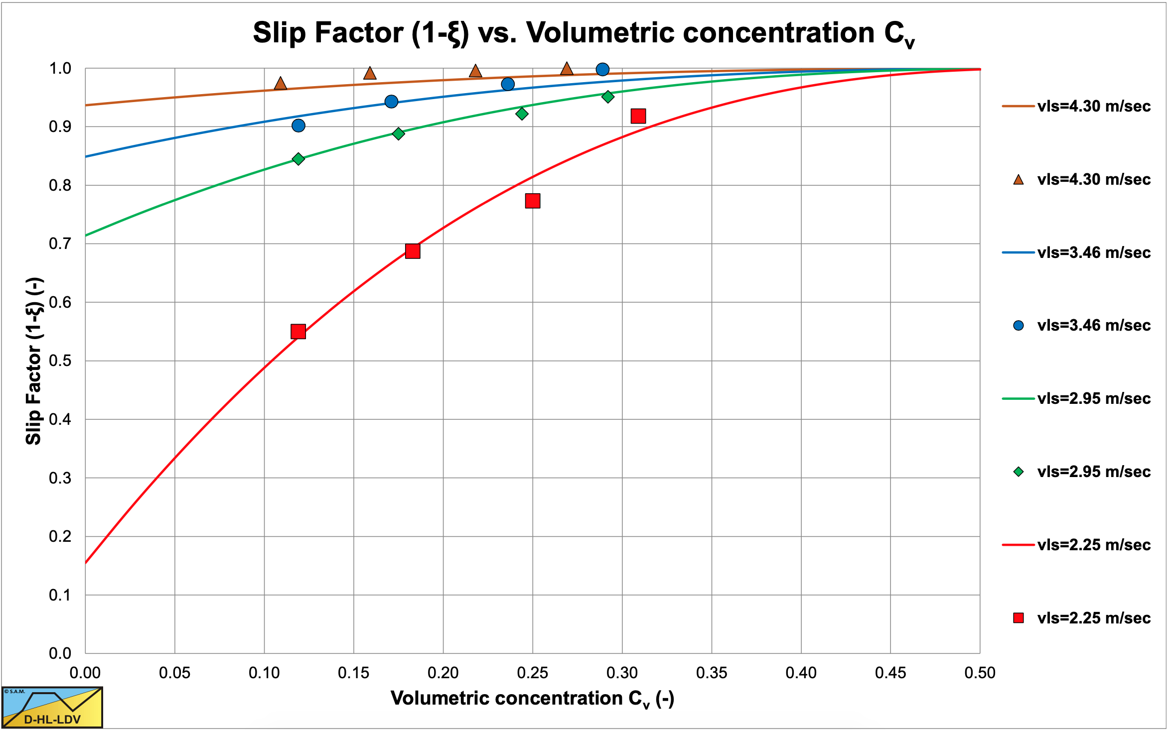
However, the experiments of Yagi et al. (1972) contain experiments at relatively low line speeds where the slip ratio tends to curve towards the asymptotic behavior at very low line speeds. In the region around the Limit Deposit Velocity a higher power may be expected. Matousek (1996) carried out experiments in a D_p=0.15 m pipe with sand with a d=0.35 mm, measuring both the volumetric spatial concentration and the volumetric delivered concentration, resulting in the slip factor (1-slip ratio). Sobota & Kril (1992) proposed an approximation correlation for the slip factor according to (source Matousek (1997)):

\[\ \frac{\mathrm{v}_{\mathrm{s}}}{\mathrm{v}_{\mathrm{l} \mathrm{s}}}=\frac{\mathrm{v}_{\mathrm{l s}}-\mathrm{v}_{\mathrm{s} \mathrm{l}}}{\mathrm{v}_{\mathrm{l s}}}=\mathrm{1}-\frac{\mathrm{v}_{\mathrm{s} \mathrm{l}}}{\mathrm{v}_{\mathrm{l s}}}=\frac{\mathrm{C}_{\mathrm{v} \mathrm{t}}}{\mathrm{C}_{\mathrm{v} \mathrm{s}}}=\mathrm{1}-\mathrm{f}_{\mathrm{t}} \cdot\left(\mathrm{1}-\frac{\mathrm{C}_{\mathrm{v s}}}{\mathrm{C}_{\mathrm{v b}}}\right)^{2.16} \cdot\left(\frac{\mathrm{v}_{\mathrm{l s}, \mathrm{ld} \mathrm{v}}}{\mathrm{v}_{\mathrm{l s}}}\right)^{\mathrm{1 .6 6}}\]

This correlation was based on results of the microscopic model of Kril (1990) for the internal structure of slurry flow. Berman (1994) determined the coefficient f_t to be:

\[\ \mathrm{f}_{\mathrm{t}}=\mathrm{0 .4 5} \cdot\left(\mathrm{1}+\operatorname{sign}\left(\ln \left(\mathrm{R} \mathrm{e}_{\mathrm{p}}\right)-\mathrm{0 .8 8}\right) \cdot \tanh \left(\mathrm{0 .9 6 7} \cdot \mathrm{a b s}\left(\ln \left(\mathrm{R} \mathrm{e}_{\mathrm{p}}\right)-\mathrm{0 .8 8}\right)^{0.6}\right)\right)\]

The 3 terms in these equations make sense. The f_t term gives the relation between the slip ratio and the particle diameter, but in a complicated way. Using the Durand drag coefficient is more transparent. The term (1-C_vs/C_vb) matches the asymptotic behavior of the theoretical slip ratio at very small line speeds with the difference that the constant spatial concentration is used here. Whether this is intentional or a typing error is not clear, but using the constant transport concentration makes more sense. The third term seems logic in the area around the Limit Deposit Velocity. The power of 1.66 seems low, but can be explained from a wide range of line speeds, see Figure 7.9-3. Both the Yagi et al. (1972) and the Matousek (1996) data point to a much higher power like 4.

Based on the Matousek (1996) experiments (see Figure 7.9-4) and the Yagi et al. (1972) experiments, the following equation is derived for the slip ratio in the region around the Limit Deposit Velocity for sand and gravel.

\[\ \frac{\mathrm{v}_{\mathrm{sl}}}{\mathrm{v}_{\mathrm{l s}}}=\frac{\mathrm{v}_{\mathrm{t}}^{2}}{\mathrm{4} \cdot \mathrm{g} \cdot \mathrm{d}} \cdot\left(\mathrm{1}-\frac{\mathrm{C}_{\mathrm{v} \mathrm{t}}}{\mathrm{C}_{\mathrm{v b}}}\right)^{2.5} \cdot\left(\frac{\mathrm{v}_{\mathrm{l s}, \mathrm{ld} \mathrm{v}}}{\mathrm{v}_{\mathrm{l s}}}\right)^{4}\]

Figure 7.9-4: The slip factor (1-slip ratio) according to Matousek (1996).

Yagi et al. (1972) found an equation of the following form.

\[\ \xi=\frac{\mathrm{v}_{\mathrm{sl}}}{\mathrm{v}_{\mathrm{ls}}}=\mathrm{A} \cdot\left(\frac{\mathrm{g} \cdot \mathrm{R}_{\mathrm{s} \mathrm{d}} \cdot \mathrm{D}_{\mathrm{p}}}{\mathrm{v}_{\mathrm{l} \mathrm{s}}^{2} \cdot \sqrt{\mathrm{C}_{\mathrm{x}}}}\right)^{\mathrm{B}}\]

Since the slip ratio at zero line speed equals (1-C_vt/C_vb) the equation is modified (later another equation is derived). For all materials the following equation is proposed:

\[\ \xi=\frac{\mathrm{v}_{\mathrm{sl}} }{\mathrm{v}_{\mathrm{ls}}}=\frac{\mathrm{R}_{\mathrm{s d}}}{\mathrm{3}} \cdot \frac{\mathrm{3}}{4} \cdot \frac{\mathrm{v}_{\mathrm{t}}^{2}}{\mathrm{g} \cdot \mathrm{R}_{\mathrm{s d}} \cdot \mathrm{d}} \cdot\left(\mathrm{1}-\frac{\mathrm{C}_{\mathrm{v} \mathrm{t}}}{\mathrm{C}_{\mathrm{v b}}}\right) \cdot\left(\frac{\mathrm{v}_{\mathrm{l s}, \mathrm{ld} \mathrm{v}}}{\mathrm{v}_{\mathrm{l} \mathrm{s}}}\right)^{4}=\mathrm{0 .3 3} \cdot \frac{\mathrm{R}_{\mathrm{s} \mathrm{d}}}{\mathrm{C}_{\mathrm{D}}} \cdot\left(\mathrm{1}-\frac{\mathrm{C}_{\mathrm{v} \mathrm{t}}}{\mathrm{C}_{\mathrm{v} \mathrm{b}}}\right) \cdot\left(\frac{\mathrm{v}_{\mathrm{l s}, \mathrm{l} \mathrm{d} \mathrm{v}}}{\mathrm{v}_{\mathrm{l} \mathrm{s}}}\right)^{4}\]

7.9.7 Comparison with the Yagi et al. (1972) Data Step 3

Comparing equation (7.9-34) with the Yagi et al. (1972) (Figure 7.9-5 & Figure 7.9-6) shows that at low concentrations the data points at the upper right are covered, while at the highest concentrations the data points in the middle and at the lower left are covered. Also the steepness of the lines match the steepness of the cloud of data points. Apparently the behavior of the slip ratio around the Limit Deposit Velocity is well described by equation (7.9-34).

Constructing the slip ratio curves according to equation (7.9-26) for the fixed bed regime, equation (7.9-34) around the Limit Deposit Velocity and equation (7.9-12) for the heterogeneous transport result in Figure 7.9-7 for low concentrations and Figure 7.9-8 for the highest concentrations. The curves match well and also show that both the lines of the sands and the gravels cover the whole area of data points which matches the findings of Yagi et al. (1972). The transition however from the fixed bed regime to the regime around the Limit Deposit Velocity is still to abrupt and tends to overestimate the slip ratio measured by Yagi et al. (1972). One more step has to be taken to smoothen this transition.

7.9.8 Construction of the Slip Ratio Curve, Step 4

Figure 7.9-10 shows how the resulting slip ratio curve is constructed. First the semi-empirical slip ratio curve based on equation (7.9-34) is drawn, which is the LDV Region slip ratio curve in the figure. Secondly the theoretical slip ratio curve for the Fixed Bed according to equation (7.9-26) is drawn. Now one could construct a resulting slip ratio curve by choosing the smallest slip ratio (of the two) at each line speed, but this results in a rather abrupt transition between the LDV Region slip ratio curve and the theoretical Fixed Bed slip ratio curve. So how to make this transition more smooth? Taking the tangent to the LDV Region slip ratio curve, starting at a slip ratio according to equation (7.9-29) could be a solution, but the results are not yet satisfactory comparing it with the experiments of Doron et al. (1987). Taking a weighted average of the LDV Region and the Fixed Bed slip ratio curve and the tangent curve, gives a good correlation as is shown in Figure 7.9-11 and Figure 7.9-12 for a 4.2% and an 18% volumetric transport concentration (Doron et al. (1987)).

Looking at Figure 7.9-7 it is clear that there are not many data points with a slip velocity higher than 50% of the line speed. So this correction does not really influence the outcome of Figure 7.9-7. Grunsven (2012) defined the slip factor as 1 minus the slip ratio as used by Yagi et al. (1972). He carried out experiments in a 40 mm Perspex pipe with sands with a d50 of 0.132 mm (GB), 0.325 mm (D9) and 0.570 mm (D8), measuring both the volumetric spatial and the volumetric transport concentration. Based on these measurements he determined the slip factor. Since these experiments are carried out independently from the experiments of Yagi et al. (1972), as used to calibrate the slip efficiency, it is interesting to compare the results of equation (7.9-12), (7.9-26) and (7.9-32) with the data of Grunsven (2012). Figure 7.9-13 shows this comparison. From this figure it can be concluded that the theory matches the experiments closely. Of course there is some scatter, but the theoretical curves of a specific sand, match the data points of that specific sand rather well. For smaller line speeds, the data points of the slip factor seem to deviate based on the concentration, matching the trend of the theoretical curves, although the data points for the lowest line speeds seem to have a smaller slip factor then predicted.

7.9.9 Conclusions & Discussion

To estimate the slip ratio 3 regions have to be distinguished, the fixed bed region at line speeds much smaller than the Limit Deposit Velocity, the region around the Limit Deposit Velocity and the heterogeneous region at line speeds higher than the Limit Deposit Velocity. For each region an equation has been derived. In order to match the theoretical curves with the data points of Yagi et al. (1972), Doron et al. (1987) and Grunsven (2012), smoothing of the transition between the fixed bed regime and the LDV regime is applied.

The resulting slip ratio curves give a good correlation with the measurements of Yagi et al. (1972), Doron et al. (1987) and Grunsven (2012). Since these experiments are carried out independently in different periods of time and under different conditions, the method described gives promising results.

Figure 7.9-5: The data of Yagi et al. (1972) compared with the theoretical slip velocities, step 3, C_vt=0.05.

Figure 7.9-6: The data of Yagi et al. (1972) compared with the theoretical slip velocities, step 3, C_vt=0.11-0.34.

Figure 7.9-7: The data of Yagi et al. (1972) compared with the theoretical slip velocities, step 3, C_vt=0.05.

Figure 7.9-8: The data of Yagi et al. (1972) compared with the theoretical slip velocities, step 3, C_vt=0.11-0.34.

Figure 7.9-9: Construction of the slip ratio curve, step 4 on linear axis.

Figure 7.9-10: Construction of the slip ratio curve, step 4 on logarithmic axis.

Figure 7.9-11: The resulting slip ratio applied to the experiments of Doron et al. (1987), C_vt=0.042-0.050.

Figure 7.9-12: The resulting slip ratio applied to the experiments of Doron et al. (1987), C_vt=0.17-0.21.

Figure 7.9-13: The slip factor, theory and experiments (data Grunsven (2012)).

Figure 7.9-14: The slip ratio and factor, the bed fraction and the spatial concentration.

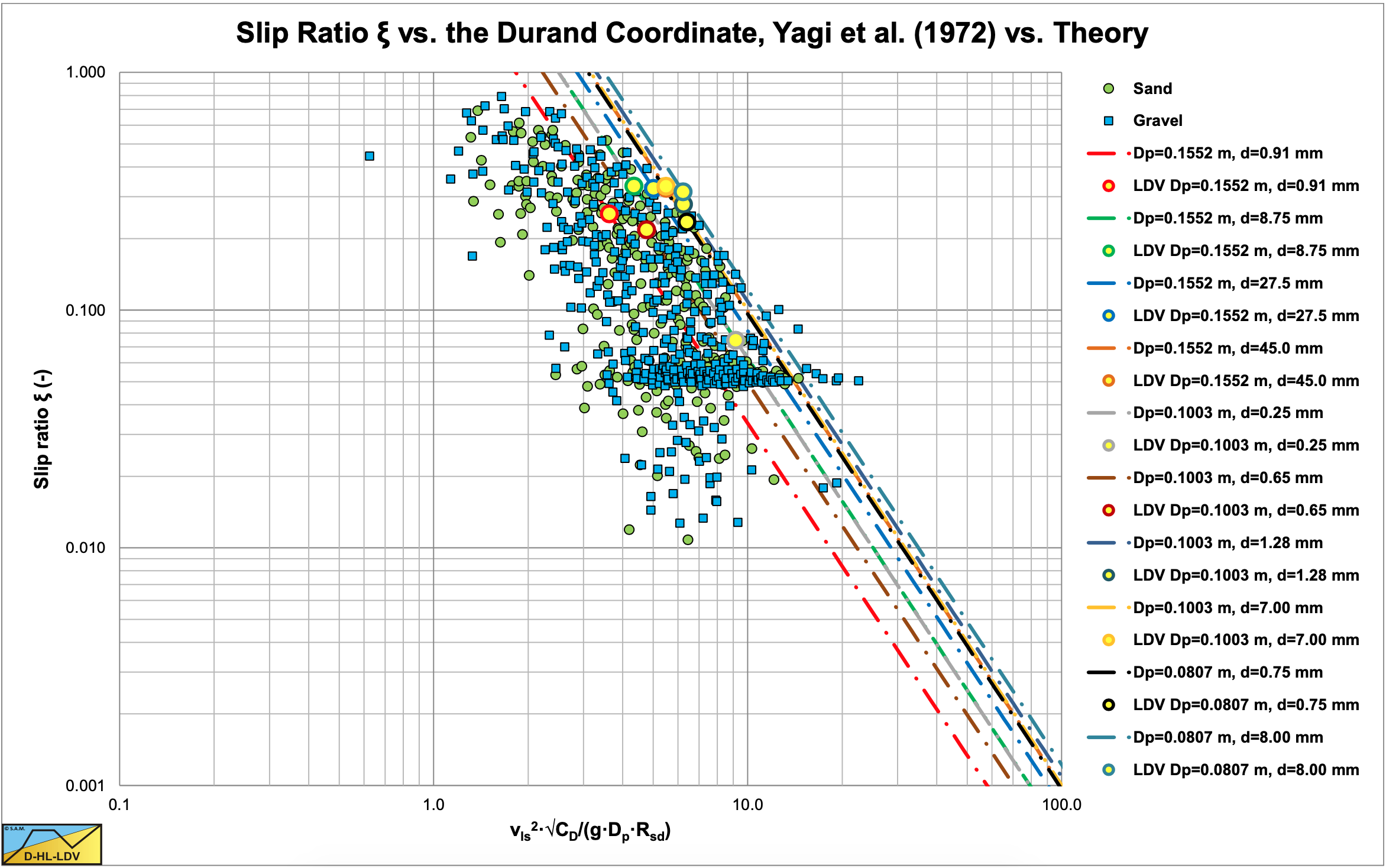
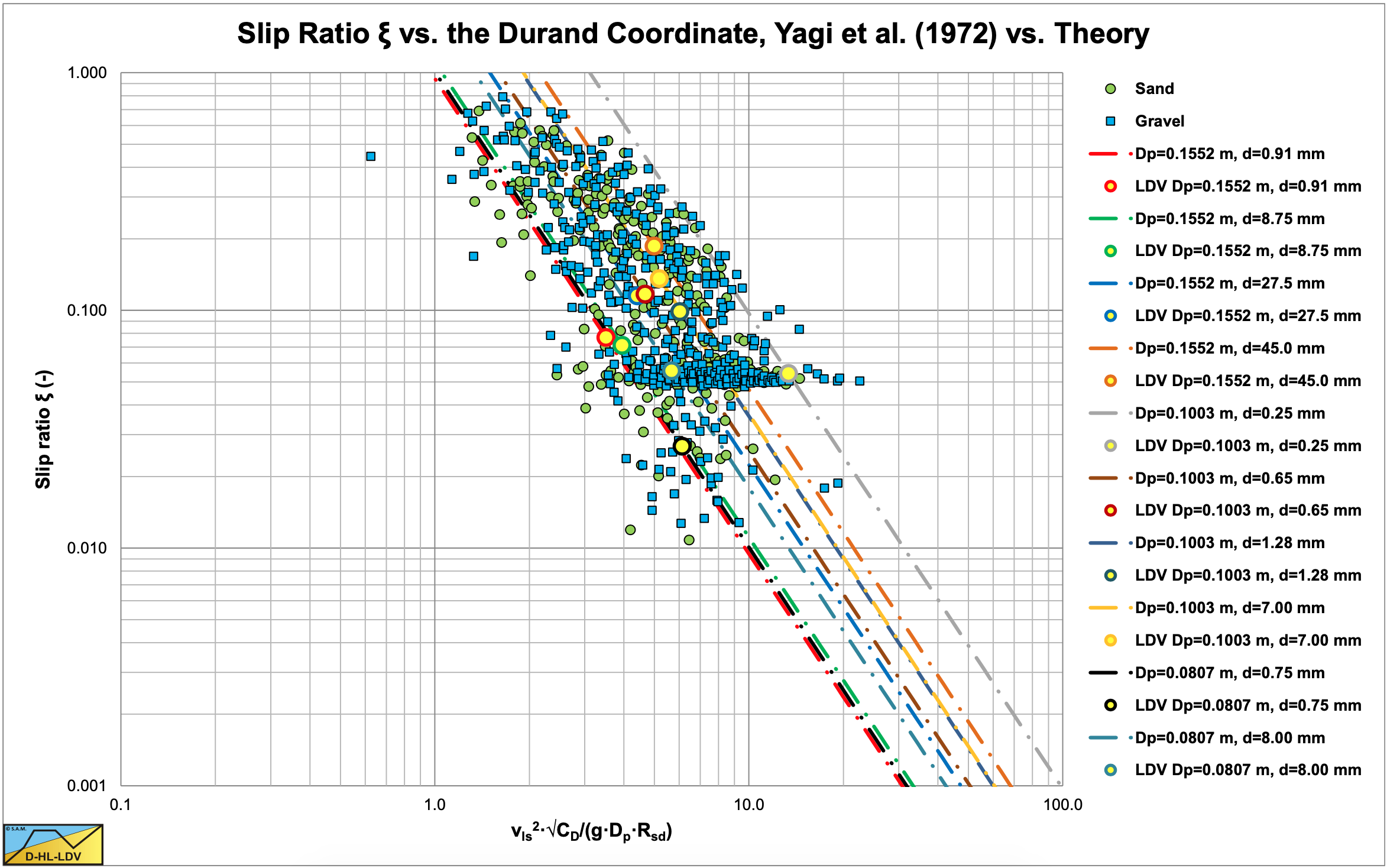
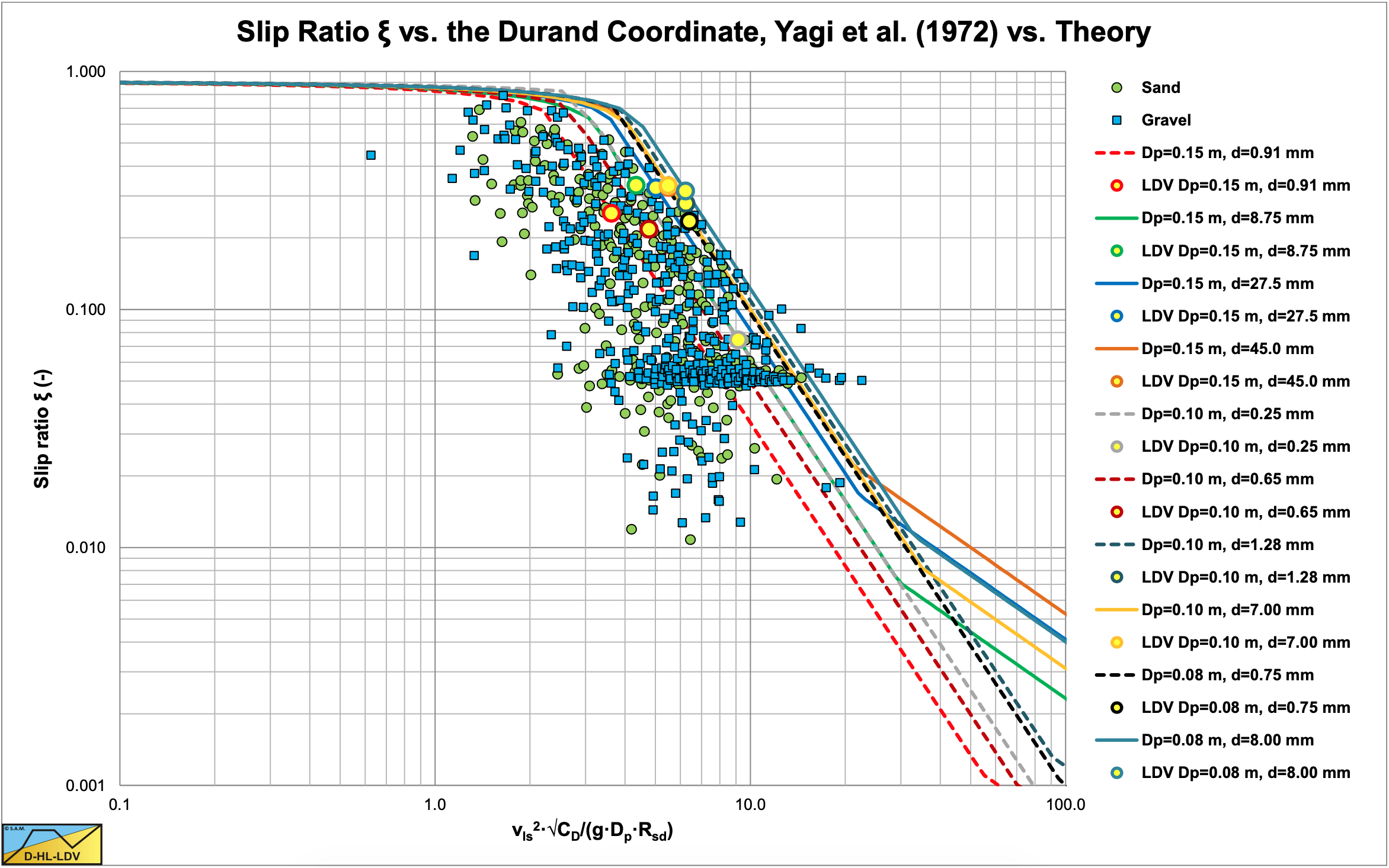
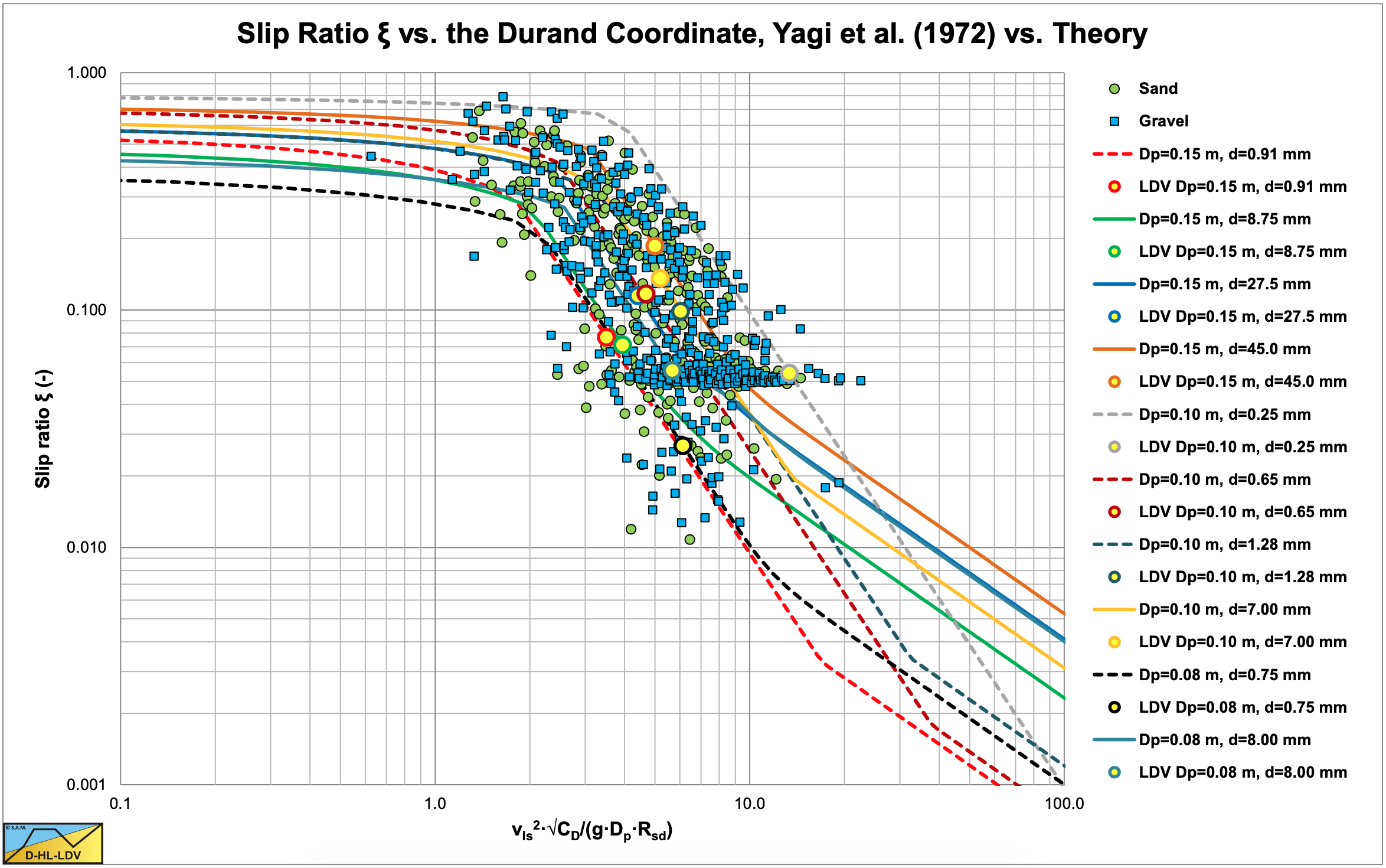
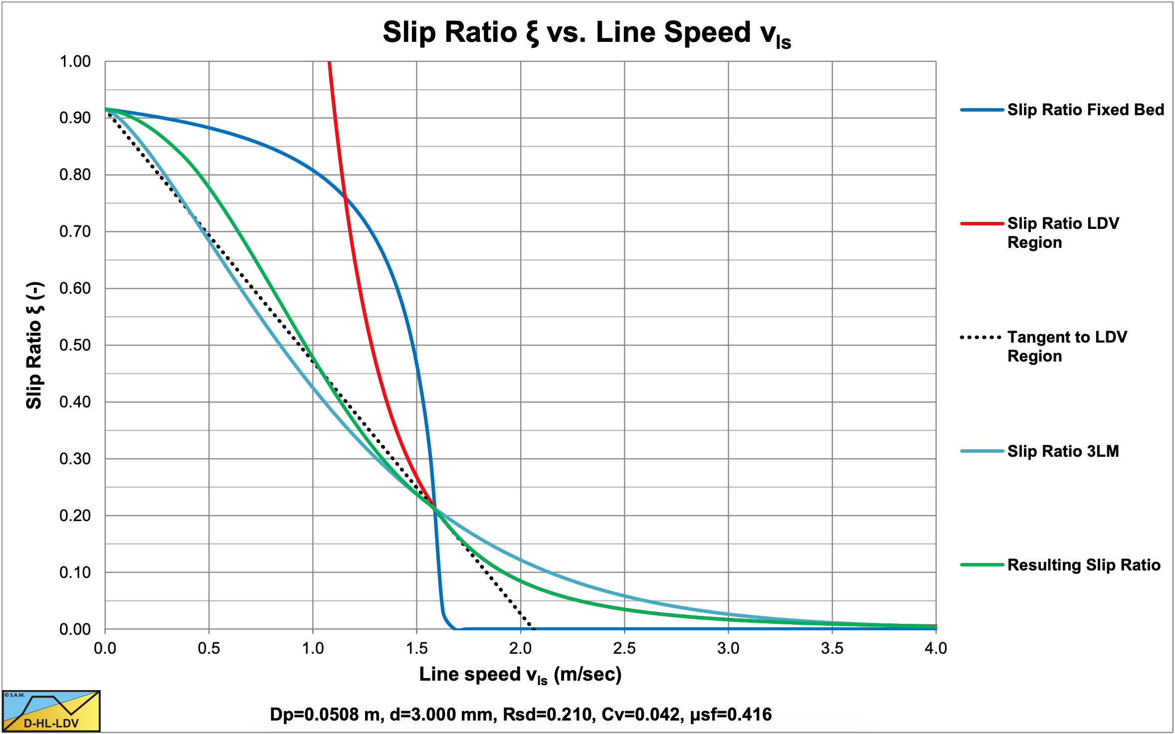
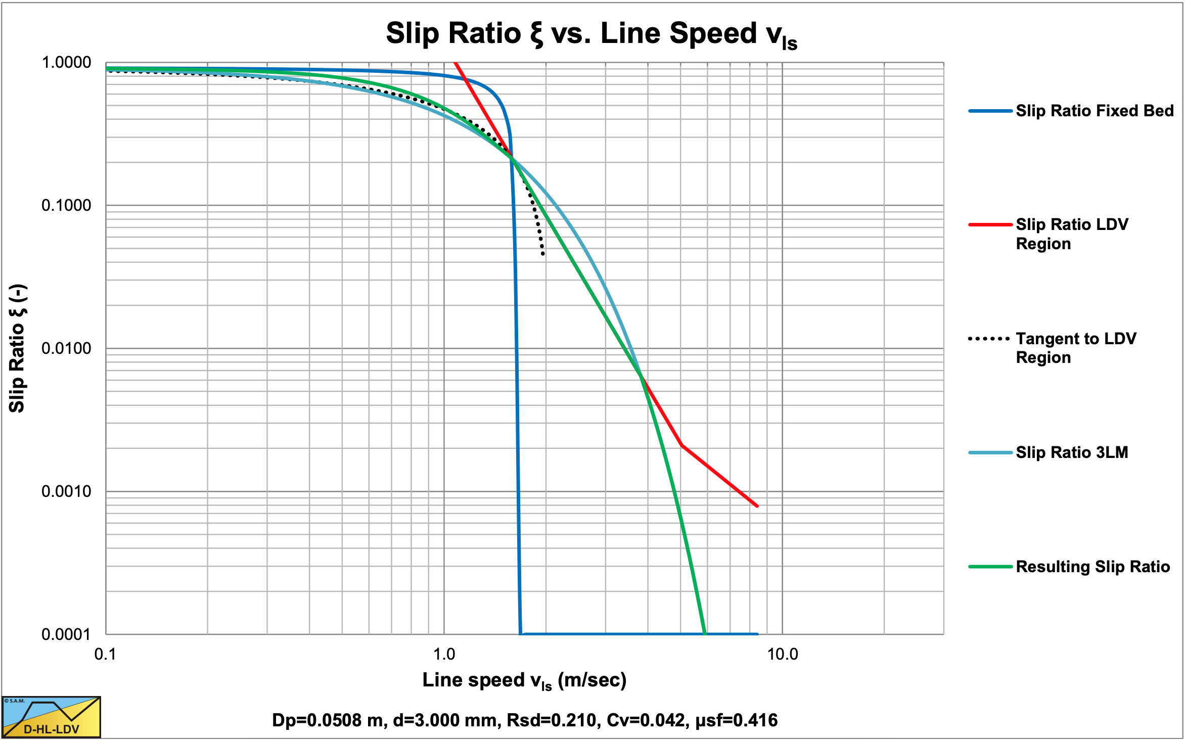
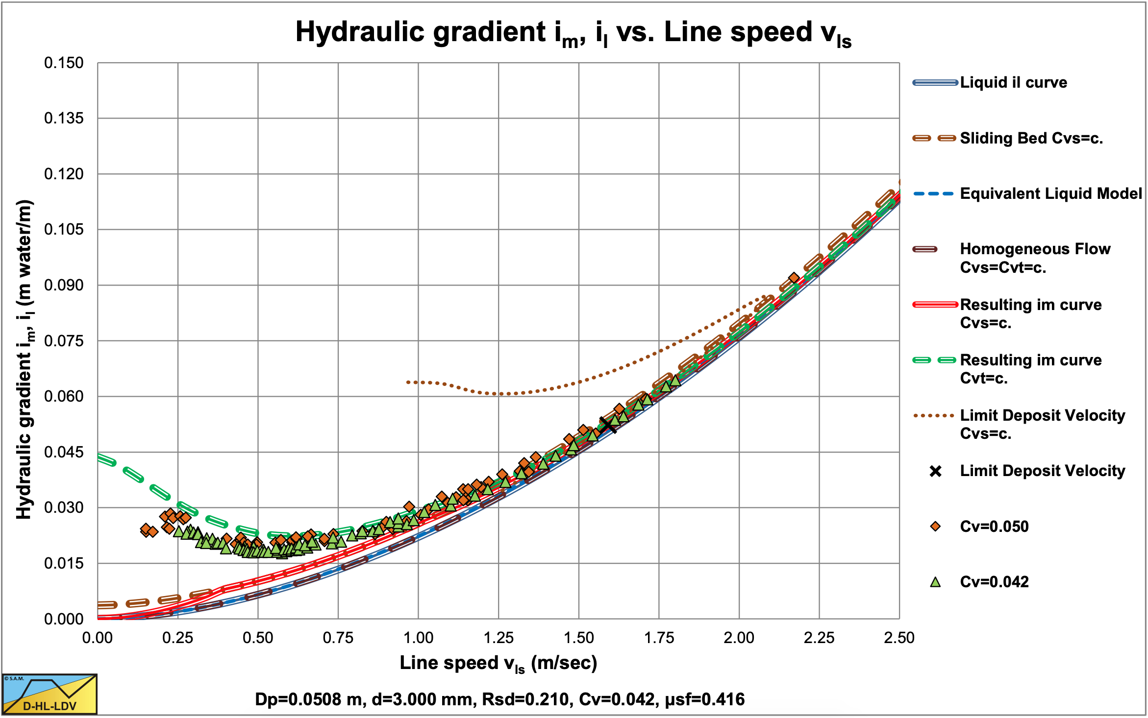
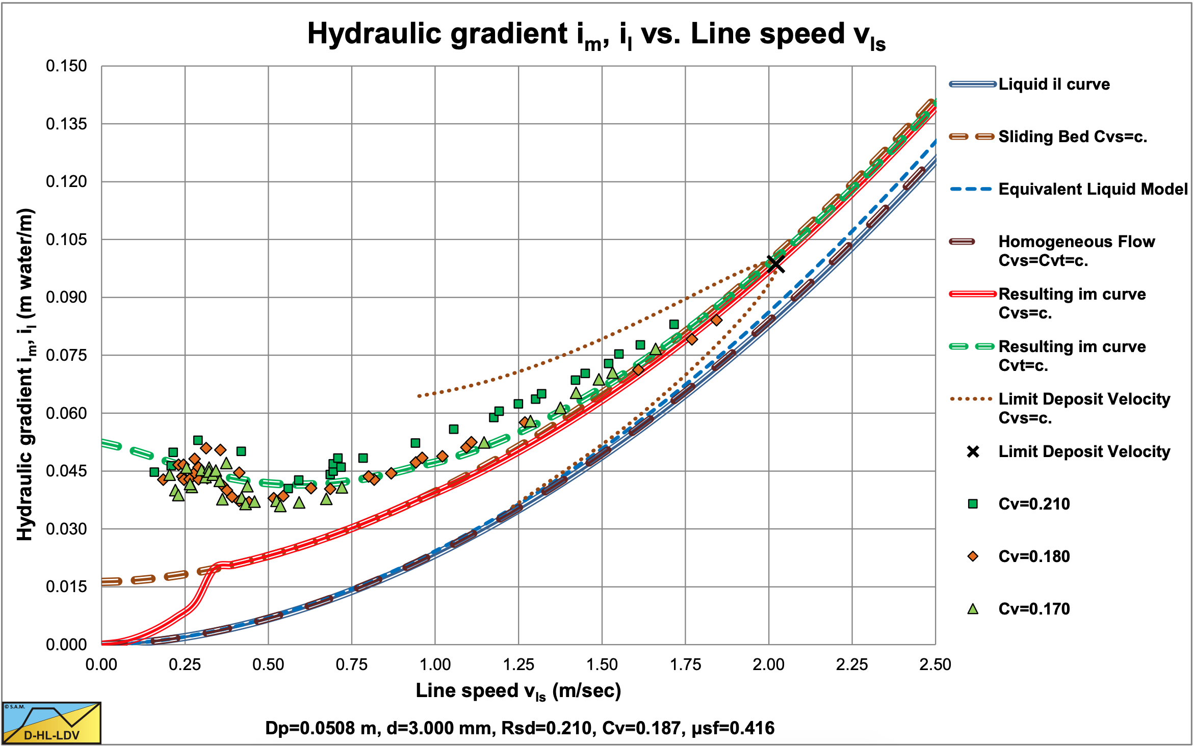
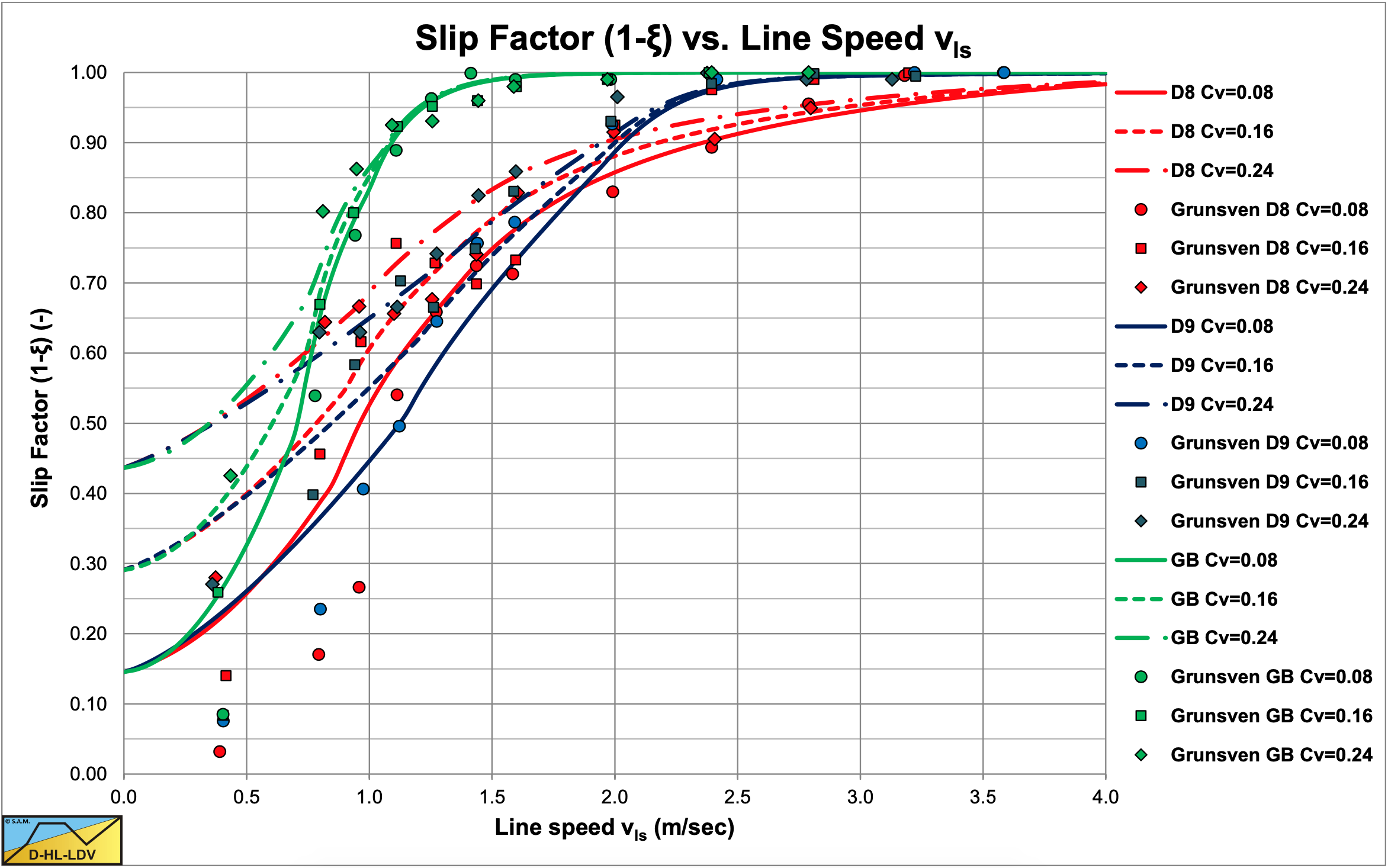
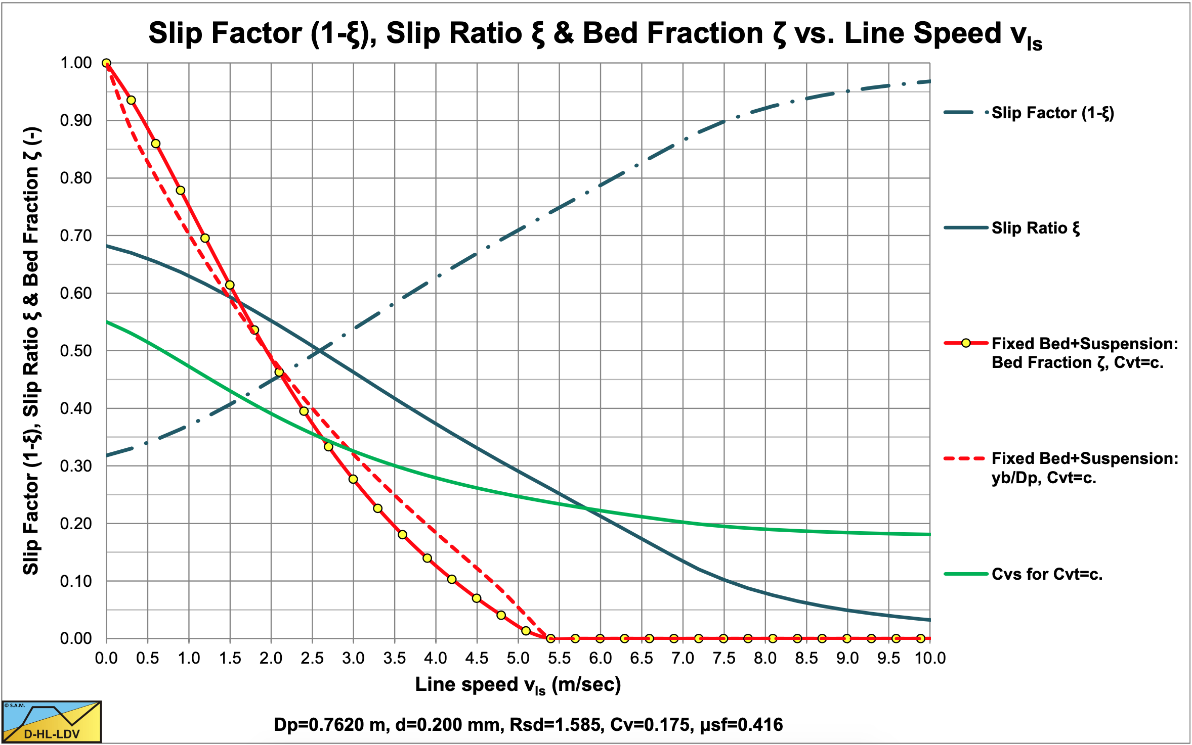
Figure 7.9-14 shows the resulting slip ratio, slip factor, bed fraction, bed height and spatial volumetric concentration in case of constant delivered volumetric concentration. The maximum spatial concentration is the bed concentration, which in the case considered is 55%.

7.9.10 The Slip Velocity, a Pragmatic Solution

There are 3 theoretical equations derived for the slip ratio, the region of line speeds below the LDV, the region of line speeds around the LDV and the region of line speeds above the LDV.

The slip ratio ξ_HeHo in the heterogeneous and homogeneous regime above the LDV is:

\[\ \xi_{\mathrm{HeHo}}=\frac{\mathrm{v}_{\mathrm{sl}}}{\mathrm{v}_{\mathrm{l s}}}=\mathrm{8 .5} \cdot\left(\frac{\mathrm{1}}{\sqrt{\lambda_{\mathrm{l}}}}\right) \cdot\left(\frac{\mathrm{v}_{\mathrm{t}}}{\sqrt{\mathrm{g} \cdot \mathrm{d}}}\right)^{\mathrm{5} / \mathrm{3}} \cdot\left(\frac{\left(v_{\mathrm{l}} \cdot \mathrm{g}\right)^{1 / 3}}{\mathrm{v}_{\mathrm{l s}}}\right) \cdot \frac{\mathrm{v}_{\mathrm{t}}}{\mathrm{v}_{\mathrm{ls}}}\]

The slip ratio ξ_ldv without suspension around the LDV can be approximated by (based on the 3LM equation (7.4-93)):

\[\ \begin{array}{left} \xi_{\mathrm{aldv}}=\frac{\mathrm{v}_{\mathrm{sl}}}{\mathrm{v}_{\mathrm{ls}}}=\left(1-\mathrm{C}_{\mathrm{vr}}\right) \cdot \mathrm{e}^{\left(-\left(\mathrm{0 . 8 3}+\frac{\mu_{\mathrm{sf}}}{4}+\left(\mathrm{C}_{\mathrm{vr}}-\mathrm{0 . 5 - 0 . 0 7 5 \cdot D _ { \mathrm { p } }}\right)^{2}+\mathrm{0 . 0 2 5} \cdot \mathrm{D}_{\mathrm{p}}\right) \cdot \mathrm{D}_{\mathrm{p}}^{0.025} \cdot\left(\frac{\mathrm{v}_{\mathrm{ls}, \mathrm{ldv}}}{\mathrm{v}_{\mathrm{ls}, \mathrm{lsdv}}}\right)^{\alpha} \cdot \mathrm{C}_{\mathrm{vr}}^{0.65} \cdot\left(\frac{\mathrm{R}_{\mathrm{sd}}}{1.585}\right)^{0.1}\right)} \cdot\left(\frac{\mathrm{v}_{\mathrm{l s}, \mathrm{l d v}}}{\mathrm{v}_{\mathrm{l s}}}\right)^{4}\\
\text{With: } \alpha=0.58 \cdot \mathrm{C_{vr}^{-0.42}}\\
\text{At the LDV: }\\
\xi_{\mathrm{ldv}}=\frac{\mathrm{v}_{\mathrm{sl}}}{\mathrm{v}_{\mathrm{ls}}}=\left(1-\mathrm{C}_{\mathrm{vr}}\right) \cdot \mathrm{e}^{\left(-\left(\mathrm{0} .83+\frac{\mu_{\mathrm{sf}}}{4}+\left(\mathrm{C}_{\mathrm{vr}}-\mathrm{0 . 5}-\mathrm{0} .075 \cdot \mathrm{D}_{\mathrm{p}}\right)^{2}+0.025 \cdot \mathrm{D}_{\mathrm{p}}\right) \cdot \mathrm{D}_{\mathrm{p}}^{0.025} \cdot\left(\frac{\mathrm{v}_{\mathrm{ls}, \mathrm{ldv}}}{\mathrm{v}_{\mathrm{ls}, \mathrm{lsdv}}}\right)^{\alpha} \cdot \mathrm{C}_{\mathrm{vr}}^{0.65} \cdot\left(\frac{\mathrm{R}_{\mathrm{sd}}}{1.585}\right)^{0.1}\right)}\end{array}\]

The slip ratio ξ_fb based on a fixed bed below the LDV is, with suspension above the bed:

\[\ \begin{array}{left} \xi_{\mathrm{fb}}=\frac{\mathrm{v}_{\mathrm{sl}}}{\mathrm{v}_{\mathrm{l s}}}=1-\frac{\mathrm{C}_{\mathrm{v t}} \cdot \mathrm{v}_{\mathrm{l s}, \mathrm{ld v}}}{\left(\mathrm{C}_{\mathrm{v b}}-\mathrm{\kappa}_{\mathrm{ldv}} \cdot \mathrm{C}_{\mathrm{v t}}\right) \cdot\left(\mathrm{v}_{\mathrm{l s}, \mathrm{l d v}}-\mathrm{v}_{\mathrm{l s}}\right)+\mathrm{\kappa}_{\mathrm{l d v}} \cdot \mathrm{C}_{\mathrm{v t}} \cdot \mathrm{v}_{\mathrm{l s}, \mathrm{l d v}}}\\
\mathrm{W i t h}: \mathrm{\kappa}_{\mathrm{l d v}}=\left(\frac{\mathrm{v}_{\mathrm{l s}, \mathrm{ld v}}}{\mathrm{v}_{\mathrm{l s}, \mathrm{l d v}}-\mathrm{v}_{\mathrm{s l}, \mathrm{l d v}}}\right)=\left(\frac{\mathrm{1}}{\mathrm{1 - \xi}_{\mathrm{l d v}}}\right)\end{array}\]

The slip ratio according to the 3LM model is:

\[\ \xi_{3 \mathrm{L M}}=\frac{\mathrm{v}_{\mathrm{s} \mathrm{l}}}{\mathrm{v}_{\mathrm{l} \mathrm{s}}}=\left(1-\mathrm{C}_{\mathrm{v r}}\right) \cdot \mathrm{e}^{\left(-\left(\mathrm{0 . 8 3 + \frac { \mu_{sf} } { 4 }}+\left(\mathrm{C}_{\mathrm{v r}}-\mathrm{0 . 5 - 0 . 0 7 5 .} \mathrm{D}_{\mathrm{p}}\right)^{2}+\mathrm{0 . 0 2 5} \cdot \mathrm{D}_{\mathrm{p}}\right) \cdot \mathrm{D}_{\mathrm{p}}^{0.025} \cdot\left(\frac{\mathrm{v}_{\mathrm{l s}}}{\mathrm{v}_{\mathrm{l s}, \mathrm{ls d v}}}\right)^{\alpha} \cdot \mathrm{C}_{\mathrm{v r}}^{\mathrm{0 . 6 5}} \cdot\left(\frac{\mathrm{R}_{\mathrm{s d}}}{\mathrm{1 . 5 8 5}}\right)^{0.1}\right)}\]

The resulting theoretical slip ratio curve is determined by:

\[\ \begin{array}{left}\xi_{\mathrm{fb}}<\xi_{\mathrm{aldv}} \Rightarrow \xi_{\mathrm{th}}=\xi_{\mathrm{fb}}\\
\xi_{\mathrm{fb}} \geq \xi_{\mathrm{aldv}} \Rightarrow \xi_{\mathrm{th}}=\xi_{\mathrm{aldv}}\\
\xi_{\mathrm{HeHo}}>\xi_{\mathrm{aldv}} \Rightarrow \xi_{\mathrm{th}}=\xi_{\mathrm{HeHo}}\end{array}\]

In reality ξ_HeHo may be larger, because the equation only covers the slip ratio required to explain the head losses, which would mean that particles always reach the line speed before being slowed down by collisions. This is not necessarily the case, resulting in a larger slip ratio. Multiplying with a factor 2 is suggested. On the other hand, the slip ratio resulting from this equation is very small and does not influence the resulting slip ratio curve much.

The resulting theoretical slip ratio curve however is based on a fixed bed for line speeds below the LDV. Maybe this is true at line speed zero, but at higher line speeds there will probably be a sliding bed, resulting in a smaller slip ratio. A method is described here to get a good estimate of the slip ratio in this region.

The tangent line to equation (7.9-36), going through the point on the vertical axis (1-C_vt/C_vb) is:

\[\ \begin{array}{left} \xi_{\mathrm{t}}=\frac{\mathrm{v}_{\mathrm{sl}} }{\mathrm{v}_{\mathrm{ls}}}=\left(1-\frac{\mathrm{C}_{\mathrm{v} \mathrm{t}}}{\mathrm{C}_{\mathrm{v} \mathrm{b}}}\right)-4 \cdot\left(1-\frac{\mathrm{C}_{\mathrm{v} \mathrm{t}}}{\mathrm{C}_{\mathrm{v} \mathrm{b}}}\right) \cdot \mathrm{e}^{\left(-\left(\mathrm{0} . \mathrm{8 3}+\frac{\mu_{\mathrm{sf}}}{4}+\left(\mathrm{C}_{\mathrm{vr}}-\mathrm{0 . 5}-\mathrm{0 . 0 7 5} \cdot \mathrm{D}_{\mathrm{p}}\right)^{2}+\mathrm{0 . 0 2 5} \cdot \mathrm{D}_{\mathrm{p}}\right) \cdot \mathrm{D}_{\mathrm{p}}^{0.025} \cdot\left(\frac{\mathrm{v}_{\mathrm{l s}, \mathrm{ldv}}}{\mathrm{v}_{\mathrm{ls}, \mathrm{l} \mathrm{sdv}}}\right)^{\alpha} \cdot \mathrm{C}_{\mathrm{vr}}^{0.65} \cdot\left(\frac{\mathrm{R}_{\mathrm{sd}}}{\mathrm{1 . 5 8 5}}\right)^{0.1}\right)\cdot \left( \frac{\mathrm{v_{ls,ldv}}}{\mathrm{v_{ls,t}}} \right)^4\cdot \left( \frac{\mathrm{v_{ls}}}{\mathrm{v_{ls,t}}} \right)}\\
\text{With : }\quad \mathrm{v}_{\mathrm{ls, t}}=\left(5 \cdot \mathrm{e}^{\left(-\left(0.83+\frac{\mu_{\mathrm{sf}}}{4}+\left(\mathrm{c}_{\mathrm{vr}}-0.5-0.075 \cdot \mathrm{D}_{\mathrm{p}}\right)^{2}+0.025 \cdot \mathrm{D}_{\mathrm{p}}\right) \cdot \mathrm{D}_{\mathrm{p}}^{0.025} \cdot\left(\frac{\mathrm{v}_{\mathrm{ls}, \mathrm{ldv}}}{\mathrm{v}_{\mathrm{ls}, \mathrm{lsdv}}}\right)^{\alpha} \cdot \mathrm{C}_{\mathrm{vr}}^{0.65} \cdot\left(\frac{\mathrm{R}_{\mathrm{sd}}}{1.585}\right)^{0.1}\right)}\right)^{1 / 4} \cdot\mathrm{v_{ls,ldv}}
\end{array}\]

Giving for the slip ratio of this tangent line:

\[\ \xi_{\mathrm{t}}=\frac{\mathrm{v}_{\mathrm{s} \mathrm{l}}}{\mathrm{v}_{\mathrm{ls}}}=\left(1-\frac{\mathrm{C}_{\mathrm{v} \mathrm{t}}}{\mathrm{C}_{\mathrm{v} \mathrm{b}}}\right) \cdot\left(1-\frac{4}{\mathrm{5}} \cdot\left(\frac{\mathrm{v}_{\mathrm{l s}}}{\mathrm{v}_{\mathrm{l s}, \mathrm{t}}}\right)\right)\]

The approximation of the slip ratio ξ up to the tangent point v_ls,t is now a weighed slip ratio according to:

\[\ \begin{array}{left}\xi_{\mathrm{SBHeHo}}=\xi_{\mathrm{th}} \cdot\left(1-\left(\frac{\mathrm{v}_{\mathrm{ls}}}{\mathrm{v}_{\mathrm{ls}, \mathrm{t}}}\right)^{\alpha}\right)+\xi_{\mathrm{t}} \cdot\left(\frac{\mathrm{v}_{\mathrm{l s}}}{\mathrm{v}_{\mathrm{l s}, \mathrm{t}}}\right)^{\alpha} &\quad \text{ if }\quad\mathrm{v}_{\mathrm{l s}}<\mathrm{v}_{\mathrm{l s}, \mathrm{t}}\\
\xi_{\text{SBHeHo} }=\xi_{\text {th }} &\quad\text{ if }\quad \mathrm{v}_{\mathrm{ls}} \geq \mathrm{v}_{\mathrm{l} \mathrm{s}, \mathrm{t}}\\
\text{With: }\quad \alpha=0-1\\
\xi_{\mathrm{SBHeHo}}>\xi_{3 \mathrm{LM}} \Rightarrow \xi_{\mathrm{SBHeHo}}=\xi_{3 \mathrm{LM}}\end{array}\]

This is shown in Figure 7.9-9 and Figure 7.9-10.

In the case of sliding flow, the slip ratio has to be corrected. A pragmatic approach to determine the relative excess hydraulic gradient in the sliding flow regime is to use a weighted average between the heterogeneous regime and the sliding bed regime. First the factor between particle size and pipe diameter is determined:

\[\ \mathrm{f}=\frac{4}{3}-\frac{1}{3} \cdot \frac{\mathrm{d}}{\mathrm{r}_{\mathrm{d} / \mathrm{D p}} \cdot \mathrm{D}_{\mathrm{p}}} \quad\text{ with: }\mathrm{0} \leq \mathrm{f} \leq \mathrm{1}\]

Secondly the weighted average slip ratio is determined:

\[\ \xi_{\mathrm{SF}}=\xi_{\mathrm{SBHeHo}} \cdot \mathrm{f}+\xi_{3 \mathrm{LM}} \cdot(1-\mathrm{f})\]

The resulting relative excess hydraulic gradient can be determined by multiplying the E_rhg curve for C_vt=C_vs with the factor 1/(1-ξ).

\[\ \mathrm{C}_{\mathrm{v s}}(\xi)=\left(\frac{\mathrm{1}}{\mathrm{1 - \xi}}\right) \cdot \mathrm{C}_{\mathrm{v t}} \quad \Rightarrow \quad \mathrm{E}_{\mathrm{r h g}, \mathrm{C v t}}=\left(\frac{\mathrm{1}}{\mathrm{1 - \xi}}\right) \cdot \mathrm{E}_{\mathrm{r h g}, \mathrm{C v s}=\mathrm{C v t}}\]

Now there are 2 cases, with constant C_vs a sliding bed is found or the fixed bed transits directly to heterogeneous transport.

Case sliding bed:

One should use the sliding bed equation also in the stationary bed range of the constant spatial volumetric concentration curve, so from line speed zero until the sliding bed curve intersects with the heterogeneous curve.

Case no sliding bed:

If the stationary bed regime curve intersects with the heterogeneous regime curve below the sliding bed curve, one should continue the heterogeneous curve with decreasing line speed, up to the intersection with the sliding bed curve and from there with decreasing line speed follow the sliding bed curve.

Applying this pragmatic solution to the Doron et al. (1987) experiments, as shown in Figure 7.9-11 and Figure 7.9-12, gives a good match.

The hydraulic gradient for the constant delivered volumetric concentration curve is now:

\[\ \mathrm{i}_{\mathrm{m}}=\mathrm{i}_{\mathrm{l}}+\mathrm{E}_{\mathrm{r h g}, \mathrm{C vt}} \cdot \mathrm{R}_{\mathrm{s d}} \cdot \mathrm{C}_{\mathrm{v t}}=\mathrm{i}_{\mathrm{l}}+\left(\frac{\mathrm{1}}{\mathrm{1}-\xi}\right) \cdot \mathrm{E}_{\mathrm{r h g}, \mathrm{C v s}=\mathrm{C v t}} \cdot \mathrm{R}_{\mathrm{s d}} \cdot \mathrm{C}_{\mathrm{v t}}\]

This gives for the pressure difference:

\[\ \Delta \mathrm{p}_{\mathrm{m}}=\Delta \mathrm{p}_{\mathrm{l}}+\rho_{\mathrm{l}} \cdot \mathrm{g} \cdot \Delta \mathrm{L} \cdot \mathrm{E}_{\mathrm{r h g}, \mathrm{C v t}} \cdot \mathrm{R}_{\mathrm{s d}} \cdot \mathrm{C}_{\mathrm{v t}}=\Delta \mathrm{p}_{\mathrm{l}}+\rho_{\mathrm{l}} \cdot \mathrm{g} \cdot \Delta \mathrm{L} \cdot\left(\frac{\mathrm{1}}{\mathrm{1 - \xi}}\right) \cdot \mathrm{E}_{\mathrm{r h g}, \mathrm{C v s}=\mathrm{C v t}} \cdot \mathrm{R}_{\mathrm{s d}} \cdot \mathrm{C}_{\mathrm{v t}}\]

7.9.11 Nomenclature Slip Velocity

Ab	Pipe cross section occupied by the bed	m^2
\(\ \hat{\mathrm{A}}_{\mathrm{b}}\)	Bed cross section divided by pipe cross section	-
Ap	Pipe cross section	m^2
As	Pipe cross section restricted area above the bed	m^2
CD	Particle drag coefficient	-
Cx	Durand particle Froude number	-
Cv	Volumetric concentration	-
Cvb	Volumetric bed concentration	-
Cvs	Volumetric spatial concentration	-
Cvt	Volumetric transport/delivered concentration	-
Cvs,s	Volumetric spatial concentration in restricted area above the bed	-
Cvt,s	Volumetric delivered concentration in restricted area above the bed	-
d	Particle diameter	m
d50	Particle diameter at which 50% by weight is smaller	m
Dp	Pipe diameter	m
Erhg,Cvt	Relative excess hydraulic gradient delivered concentration	-
Erhg,Cvs=Cvt	Relative excess hydraulic gradient spatial concentration	-
ft	Slip function Berman	-
g	Gravitational constant 9.81 m/s^2	m/s^2
i	Hydraulic gradient	m/m
im	Hydraulic gradient mixture	m/m
il	Hydraulic gradient water/liquid, based on viscous friction	m/m
is,pot	Hydraulic gradient potential energy losses	m/m
is,kin	Hydraulic gradient kinetic energy losses	m/m
K	Durand constant (85/181)	-
ΔL	Length of the pipeline	-
Δp	Head loss over a pipeline length ΔL	kPa
Δpm	Head loss of mixture over a pipeline length ΔL	kPa
Δpl	Head loss of liquid/water over a pipeline length ΔL	kPa
Δps,kin	Pressure required to compensate for kinetic energy losses	kPa
Δps,pot	Pressure required to compensate for potential energy losses	kPa
Rsd	Relative submerged density	-
Rsd,q	Relative submerged density quarts	-
Rsdr	Relative submerged density/Relative submerged density quarts	-
vl	Liquid velocity in pipe	m/s
vls	Line speed	m/s
vls,ldv	Limit Deposit Velocity	m/s
vp, vs	Particle velocity in direction of average flow	m/s
vsl	Slip velocity	m/s
vsl,ldv	Slip velocity at the LDV	m/s
vsl,real	Real slip velocity	m/s
vsl,real,c	Real slip velocity, corrected	m/s
vls,t	Line speed at tangent point	m/s
vt	Terminal settling velocity of particles	m/s
α-α13	Model coefficients	-
β	Power of Richardson & Zaki equation	-
κC	Concentration eccentricity factor	-
κ	Ratio Cvs to Cts	-
κldv	Ratio Cvs to Cts at the LDV	-
ρl	Liquid/liquid density	ton/m^3
ρw	Density of water	ton/m^3
ρs	Density of solids	ton/m^3
ρq	Density of quarts (2.65 ton/m^3)	ton/m^3
λ	Darcy-Weisbach friction factor	-
λl	Darcy-Weisbach friction factor liquid with pipe wall	-
μsf	Friction coefficient for sliding bed (see also Srs)	-
Φ	Durand relative excess pressure coefficient	-
Ω	Excess pressure factor	(m/s)^3
ψ	Durand abscissa	-
\(\ v_{\mathrm{w}},v_{\mathrm{l}}\)	Kinematic viscosity of water/liquid	m^2/s
ξ	Slip ratio vsl/vls	-
ξ0	Slip ratio at line speed zero	-
ξldv	Slip ratio vsl/vls at the LDV	-
ξfb	Slip ratio considering a fixed bed	-
ξHeHo	Slip ratio at high line speeds	-
ξth	Theoretical slip ratio	-
ξt	Slip ratio tangent line	-
ζ	Fraction of the pipe occupied by the sediment (bed)	-
ηsl	Slip efficiency	-
Frp	Particle Froude number of the particle settling velocity	-
Refl	Reynolds number of the slurry flow	-
Rep	Reynolds number of the particle terminal settling velocity	-
Ct	The Cát number (sand grains)	-
Th	The Thủy number (water)	-
La	The Lắng number (sediment)	-