
8.14: The Concentration Distribution
- Page ID
- 32295

The fraction can be determined by the angle β matching a certain vertical coordinate, similar to the angle β for the stationary and sliding bed.
\[\ \beta=\operatorname{acos}\left(\frac{0.5-\frac{\mathrm{r}}{\mathrm{D_{p}}}}{0.5}\right) \Leftrightarrow \frac{\mathrm{r}}{\mathrm{D_{p}}}=\frac{1-\cos (\beta)}{2}\]
The fraction f is now:
\[\ \mathrm{f}=\frac{\beta-\sin (\beta) \cdot \cos (\beta)}{\pi}\]
The concentration distribution is (without or with hindered settling):
\[\ \mathrm{C}_{\mathrm{v s}}(\mathrm{f})=\mathrm{C}_{\mathrm{v B}} \cdot \mathrm{e}^{-\frac{\alpha_{\mathrm{sm}}}{\mathrm{C}_{\mathrm{vr}}} \cdot\left(\frac{\mathrm{v}_{\mathrm{ls}, \mathrm{l} \mathrm{d v}}}{\mathrm{v}_{\mathrm{ls}}}\right)^{0.925} \cdot \frac{\mathrm{v}_{\mathrm{tv}}}{\mathrm{v}_{\mathrm{tv}, \mathrm{ld v}}} \cdot \mathrm{f}}{\quad \text{or}\quad} \mathrm{C}_{\mathrm{v s}}(\mathrm{f})=\mathrm{C}_{\mathrm{v B}} \cdot \mathrm{e}^{-\frac{\alpha_{\mathrm{sm}}}{\mathrm{C}_{\mathrm{vr}}} \cdot\left(\frac{\mathrm{v}_{\mathrm{ls}, \mathrm{ld v}}}{\mathrm{v}_{\mathrm{ls}}}\right)^{0.925} \cdot \frac{\mathrm{v}_{\mathrm{thv}}}{\mathrm{v}_{\mathrm{th v,ldv}}}\cdot\mathrm{f}}\]
The correction factor appears to depend only on the relative concentration Cvr accordoing to:
\[\ \alpha_{\mathrm{sm}}=0.9847+0.304 \cdot \mathrm{C}_{\mathrm{vr}}-1.196 \cdot \mathrm{C}_{\mathrm{vr}}^{2}-0.5564 \cdot \mathrm{C}_{\mathrm{vr}}^{3}+0.47 \cdot \mathrm{C}_{\mathrm{vr}}^{4}\]
The bottom concentration is now (without or with hindered settling):
\[\ \mathrm{C_{vB}=C_{vb}\cdot \frac{\left(\alpha_{sm}\cdot \left(\frac{v_{ls,ldv}}{v_{ls}} \right)^{0.925}\cdot \frac{v_{tv}}{v_{tv,ldv}} \right)}{\left(1-e^{\frac{\alpha_{sm}}{C_{vr}}\cdot \left(\frac{v_{ls,ldv}}{v_{ls}} \right)^{0.925}\cdot \frac{v_{tv}}{v_{tv,ldv}}}\right)}\text{ or }C_{vB}=C_{vb}\cdot\frac{\left(\alpha_{sm}\cdot\left(\frac{v_{ls,ldv}}{v_{ls}} \right)^{0.925}\cdot \frac{v_{thv}}{v_{thv,ldv}} \right)}{\left(1-e^{-\frac{\alpha_{sm}}{C_{vr}}\cdot \left(\frac{v_{ls,ldv}}{v_{ls}} \right)^{0.925}\cdot \frac{v_{thv}}{v_{thv,ldv}}} \right)}} \]
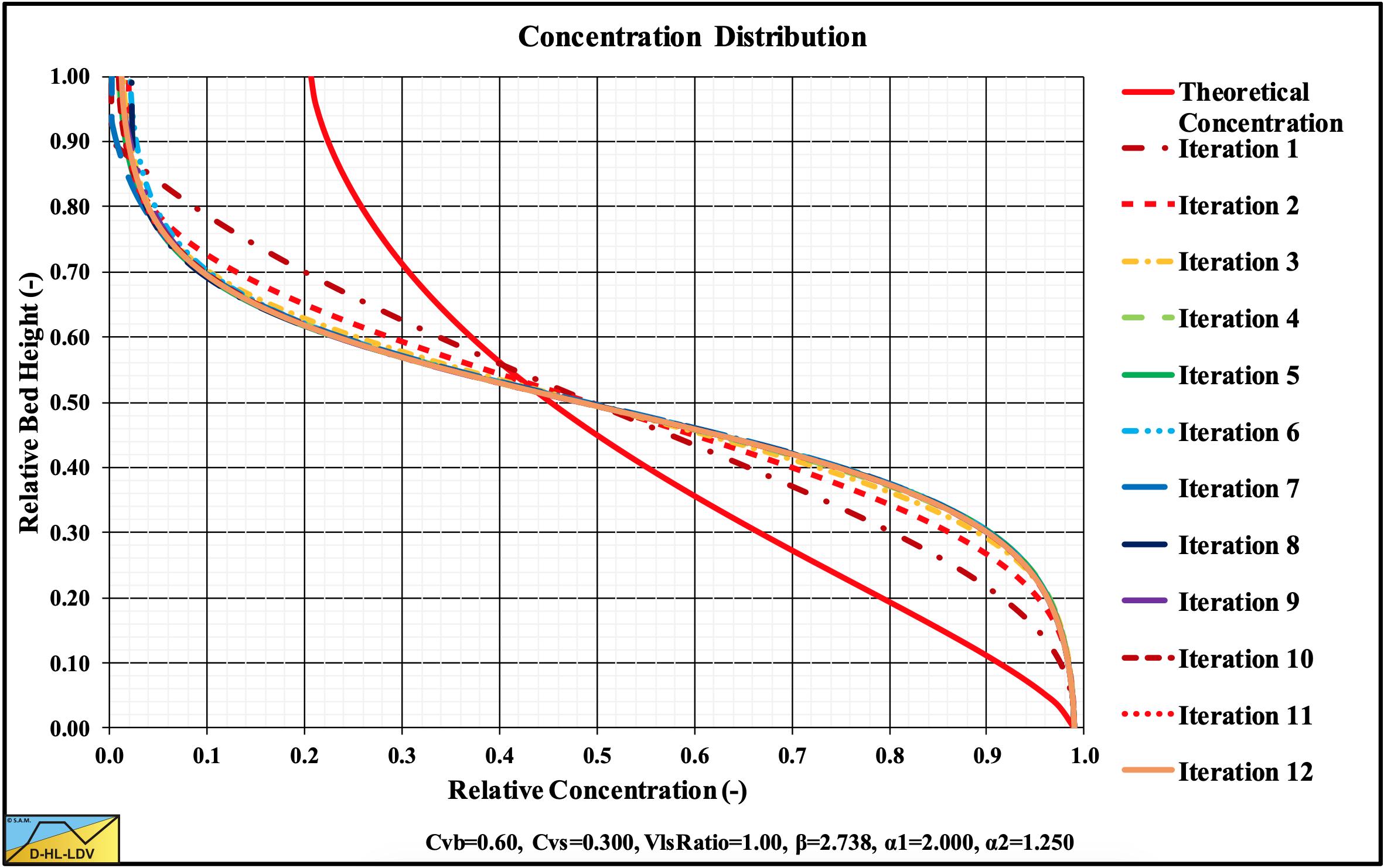
If the bottom concentration is higher than the bed concentration, the concentration profile has to be adjusted. If it is assumed that the settling velocity in the suspension hardly changes as a function of the line speed, the equation for the concentration distribution becomes:
\[\ \mathrm{C}_{\mathrm{v s}, \mathrm{0}}(\mathrm{f})=\mathrm{C}_{\mathrm{v} \mathrm{B}} \cdot \mathrm{e}^{-\frac{\mathrm{\alpha}_{\mathrm{s m}}}{\mathrm{C}_{\mathrm{v r}}} \cdot\left(\frac{\mathrm{v}_{\mathrm{ls}, \mathrm{ld v}}}{\mathrm{v}_{\mathrm{l s}}}\right)^{1.15}\cdot \mathrm{f}}\]
The bottom concentration is now:
\[\ \mathrm{C}_{\mathrm{v B}}=\mathrm{C}_{\mathrm{v b}} \cdot \frac{\left(\alpha_{\mathrm{s m}} \cdot\left(\frac{\mathrm{v}_{\mathrm{l s}, \mathrm{ld} \mathrm{v}}}{\mathrm{v}_{\mathrm{l s}}}\right)^{1.15}\right)}{\left(1-\mathrm{e}^{-\frac{\alpha_{\mathrm{sm}}}{\mathrm{C}_{\mathrm{vr}}} \cdot\left(\frac{\mathrm{v}_{\mathrm{ls}, \mathrm{ldv}}}{\mathrm{v}_{\mathrm{ls}}}\right)^{1.15}}\right)}\]
At each level in the pipe the corrected concentration gradient can be determined for the first iteration step according to:
\[\ \left(\frac{\mathrm{d} \mathrm{C}_{\mathrm{v s}, \mathrm{1}}(\mathrm{f})}{\mathrm{d r}}\right)=\left(\frac{\mathrm{d} \mathrm{C}_{\mathrm{v s}, \mathrm{0}}(\mathrm{f})}{\mathrm{d r}}\right) \cdot\left(\frac{\left(1-\mathrm{C}_{\mathrm{v r}, 0}\right)}{\left(1-\mathrm{C}_{\mathrm{v r}}\right)}\right)^{\alpha \cdot \frac{\beta}{2.34}}\]
For the following iteration steps the concentration gradient has to be adjusted according to:
\[\ \left(\frac{\left.\mathrm{d} \mathrm{C}_{\mathrm{v} \mathrm{s}, \mathrm{i}} \mathrm{(} \mathrm{f}\right)}{\mathrm{d r}}\right)=\left(\frac{\left.\mathrm{d} \mathrm{C}_{\mathrm{v s}, \mathrm{i}-\mathrm{1}} \mathrm{( f}\right)}{\mathrm{d} \mathrm{r}}\right) \cdot\left(\frac{\mathrm{C}_{\mathrm{v r}, \mathrm{i}-\mathrm{1}}(\mathrm{f})}{\mathrm{C}_{\mathrm{v r}, \mathrm{i}-\mathrm{2}}(\mathrm{f})}\right) \cdot\left(\frac{\left(1-\mathrm{C}_{\mathrm{v} \mathrm{r}, \mathrm{i}-1}\right)}{\left(1-\mathrm{C}_{\mathrm{v r}, \mathrm{i}-2}\right)}\right)^{\alpha \cdot \frac{\beta}{2.34}}\]
Integrating the concentration profile again, starting at the bottom with either the bottom concentration (above the LDV) or the bed concentration (below the LDV), gives a concentration profile adjusted for local hindered settling. The power α is determined with the following equations:
\[\ \begin{array}{left}\text{SF = Shape Factor} \quad \text{SF=0.77 for sand} \quad \text{SF=1.0 for spheres}\\
C_{\text {vrMax }}=\frac{0.175}{\mathrm{C_{v b}}}\\
\alpha=0.275 \cdot\left(\frac{\mathrm{SF}}{0.77}\right)^{1.5} \cdot\left(\frac{\mathrm{C}_{\mathrm{vr}}}{\mathrm{C}_{\mathrm{vrMax}}}\right)^{3} \cdot\left(\frac{\mathrm{v}_{\mathrm{ls}, \mathrm{LDV}}}{\mathrm{v}_{\mathrm{ls}}}\right)^{0.15} \quad \mathrm{C}_{\mathrm{vr}}<\mathrm{C}_{\mathrm{vrMax}}\\
\alpha=0.275 \cdot\left(\frac{\mathrm{SF}}{0.77}\right)^{1.5} \cdot\left(\frac{\mathrm{C}_{\mathrm{vr}}}{\mathrm{C}_{\mathrm{vrMax}}}\right)^{2 / 3} \cdot\left(\frac{\mathrm{v}_{\mathrm{ls}, \mathrm{LDV}}}{\mathrm{v}_{\mathrm{ls}}}\right)^{0.15} \quad \mathrm{C}_{\mathrm{vr}} \geq \mathrm{C}_{\mathrm{vrMax}}\end{array}\]
Because the Limit Deposit Velocity is based on the occurrence of some bed at the bottom of the pipe, this bed does not need to have the maximum bed density. A bed may start to occur with a bottom concentration of about 50%, while the maximum bed concentration will be in the range of 60%-65%. In order to find a bottom concentration of about 50% at the LDV, an additional velocity ratio rLDV is introduced giving:
\[\ \mathrm{C_{vB}=C_{vb}\cdot \frac{\left(\alpha_{sm}\cdot\left(r_{LDV}\cdot \frac{v_{s,ldv}}{v_{ls}} \right)^{1.15}\right)}{\left(1-e^{-\frac{\alpha_{sm}}{C_{vr}}\cdot \left(r_{LDV}\cdot\frac{v_{ls,ldv}}{v_{ls}} \right)^{1.15}}\right)} \quad\text{and}\quad C_{vs}(f)=C_{vB}\cdot e^{-\frac{\alpha_{sm}}{C_{vr}}\cdot \left(r_{LDV \cdot \frac{v_{ls,ldv}}{v_{ls}}} \right)^{1.15}\cdot f}}\]
The additional velocity ratio rLDV can be estimated by:
\[\ \begin{array}{left}\text{SF = Shape Factor} \quad \text{SF=0.77 for sand} \quad \text{SF=1.0 for spheres}\\
\mathrm{C_{\text {vrMax }}=\frac{0.175}{C_{v b}}}\\
\mathrm{\alpha_{\beta}=1.8-56 \cdot v_{t} \quad\text{ with: }\quad \alpha_{\beta} \geq 1.1}\\
\text{If }\mathrm{C}_{\mathrm{v r}}<\mathrm{C}_{\mathrm{v r} \mathrm{M a x}}\text{ then}\\
\mathrm{r_{L D V}=0.6 \cdot \frac{e^{(\beta / 2.34)^{\alpha_{\beta}}}}{e} \cdot\left(\frac{0.0005}{d}\right)^{S F^{6}} \cdot\left(\frac{C_{v r M a x}}{C_{v r}}\right)^{1 / 3} \quad\text{ with: }\quad r_{L D V} \geq 1.2 \cdot\left(\frac{C_{v r M a x}}{C_{v r}}\right)^{1 / 3}}\\
\text{If }\mathrm{C}_{\mathrm{v r}} \geq \mathrm{C}_{\mathrm{v r} \mathrm{M a x}}\text{ then}\\
\mathrm{r_{L D V}=0.6 \cdot \frac{e^{(\beta / 2.34)^{\alpha_{\beta}}}}{e} \cdot\left(\frac{0.0005}{d}\right)^{S F^{6}} \cdot\left(\frac{C_{v r}}{C_{v r M a x}}\right)^{1 / 6} \quad\text{ with: }\quad r_{L D V} \geq 1.2 \cdot\left(\frac{C_{v r}}{C_{v r M a x}}\right)^{1 / 6}}\end{array}\]
The factor 1.2 is based on the ratio 60% to 50%, the maximum bed concentration to the minimum bed concentration. For most of the experimental data analysed, a maximum bed concentration of 60% gives very good results. The LDV has a maximum at a concentration of 17.5%.