9.5: Comparison Graded Sands and Gravels

9.5.1 Introduction

Most slurry transport models in literature are based on a uniform Particle Size Diagram (PSD). So, all the particles have the same size. The experiments on which these models are based were carried out with either a narrow graded PSD or a uniform PSD. Most empirical models are also based on the delivered volumetric concentration, since that is what was measured. The more fundamental 2LM and 3LM models are based on a uniform PSD and a spatial volumetric concentration. Delivered concentration curves are achieved by interpolation of delivered concentrations derived from slip ratios. For non-uniform graded or broad graded PSD’s the problem is, that the interaction between the different fractions is not known. So, one can assume there is no interaction, all fractions behave independently, or one can assume a certain interaction between the fractions. The models considered here have some interaction.

The models of Durand & Condolios (1952) and Wilson et al. (1992) are both based on an adjustment of the equation for the heterogeneous flow regime, but in different ways. Durand & Condolios (1952) assume the particle Froude number has to be weighted based on a parallel resistor method, leaving the power of the line speed in the equation -1. So, the pressure losses and the hydraulic gradient are reversely proportional to the line speed. This model always gives a reduction of the solids effect. For the Durand & Condolios (1952) model one can also define a v₅₀, if the sliding friction coefficient μ_sf is known. However, this v₅₀ will change with the grading.

Wilson et al. (1992) assume that the v₅₀, the line speed where 50% stratification occurs, does not change because of the grading. However, the proportionality of the pressure losses and the hydraulic gradient changes. Uniform PSD’s are reversely proportional to the line speed with a power of 1.7 (the maximum power), medium graded PSD’s are reversely proportional to the line speed to a power around 1 and very broad graded PSD’s are reversely proportional to the line speed with a power of 0.25 (the minimum power).

Comparing the two models one can say that in the Durand & Condolios (1952) model the v₅₀ decreases with increasing grading of the PSD, with a constant proportionality of the pressure losses and the hydraulic gradient with the line speed, while the Wilson et al. (1992) model keeps the v₅₀ constant, but changes the proportionality of the pressure losses and the hydraulic gradient with the line speed.

Where the previous two models are based on heterogeneous transport only, the other three models are based on a combination of different flow regimes.

The Sellgren & Wilson (2007) 4 component model divides the PSD in 4 components based on particle size boundaries. These components are:
Homogeneous flow (the fines d<0.04 mm).
Pseudo homogeneous flow (0.04 mm<d<0.2· \(\ v_{\mathrm{r}}\) mm).
Heterogeneous flow (0.2·\(\ v_{\mathrm{r}}\) mm<d<0.015·D_p).
Fully stratified flow (d>0.015·D_p).
The first boundary from homogeneous to pseudo homogeneous flow is fixed. The second boundary from pseudo homogeneous to heterogeneous flow only depends on the relative viscosity of the carrier liquid, so for clear water it is also fixed. The third boundary from heterogeneous to fully stratified flow depends on the pipe diameter. By splitting up the PSD in the 4 fractions, determining the hydraulic gradient as a function of the line speed for each fraction and adding up the weighed hydraulic gradient curves found, the hydraulic gradient curve of the entire PSD is found. In this method, some adjustments are made for concentrations and relative submerged densities, based on the assumed properties of the carrier liquid. Any dependency of the line speed on the boundaries between the different components is not present in this model. The interactions between the fractions are based on the viscosity and density of the homogeneous carrier liquid and the resulting relative submerged density of the coarser components.

As an alternative to the 4CM the author combined the different Wilson flow regime models into a Wilson 4 regime model (4RM). The flow regimes are the homogeneous flow regime where very small particles influence the viscosity and the density of the carrier liquid creating a pseudo liquid, the stratified flow regime, the heterogeneous flow regime and the homogeneous flow regime at very high line speeds. The last 3 flow regimes use the adjusted properties of the carrier liquid. The PSD is also adjusted, since the fines now are part of the carrier liquid. If the stratified flow regime gives a smaller hydraulic gradient than the heterogeneous flow regime, the stratified flow regime is chosen, otherwise the heterogeneous flow regime. The transition of the heterogeneous flow regime to the homogeneous flow regime is determined based on the so-called stratification ration. If a certain percentage of the particles is stratified, then 1 minus this percentage is in suspension.

The DHLLDV Framework of Miedema (June 2016) includes all flow regimes depending on the particle size of a fraction. First the homogeneous fraction is determined, based on a Stokes number. The carrier liquid properties are adjusted based on the homogeneous fraction, both the viscosity and the density. For all other particles, it is assumed they are transported by this new homogeneous pseudo liquid. Until here the model is similar to the 4- component model, except for the value of the boundary. When the homogeneous fraction is known, the PSD of the remaining particles can be constructed. This PSD is divided into a number of fractions. This number can be any number; however, 9 fractions is sufficient in most cases. For each fraction the hydraulic gradient curve is determined, including all flow regimes that may occur, from line speed zero to some maximum, for example 10 m/s, depending on the pipe diameter. Both hydraulic gradient curves for spatial and delivered volumetric concentration are determined. The hydraulic gradient curves are summed based on the percentage of each fraction in the modified PSD, resulting in a constant spatial volumetric concentration curve and a constant delivered volumetric concentration curve. By multiplying the resulting curves with the ratio of the pseudo liquid density to the water density, the hydraulic gradient curves with respect to water are found. Here the boundaries between the flow regimes are not fixed, but depend on the line speed, the particle diameter and the pipe diameter.

Good methods should match the following requirements:

• The resulting hydraulic gradient curve has to match experimental data.
• The PSD should be based on the spatial situation; the delivered PSD follows.
• The method should give continuous results with respect to particle diameter and line speed.
• The method should converge to the uniform model for narrow graded PSD’s.

Before discussing the 5 models in detail, a method is given to determine a PSD and how to determine the pseudo liquid properties.

9.5.2 A Method to Generate a PSD

In order to compare the different models a Particle Size Diagram (PSD) has to be generated. The original fractions of the PSD can be determined manually by sieve analysis, or generated based on for example the d₅₀/d₁₅ and d₈₅/d₅₀ ratios. A mathematical function describing the shape of a PSD up to the d₅₀ is:

\[\ \begin{array}{left} \left(\mathrm{f}_{\mathrm{y}}=\frac{\mathrm{1}}{\mathrm{1}+\mathrm{e}_{\mathrm{x}}^{\mathrm{A_x}\cdot\left(\frac{\log 10\left(\mathrm{d}_{\mathrm{y}}\right)}{\log 10\left(\mathrm{d}_{50}\right)}-1\right)}}\right)\\
\text{with: }\quad \mathrm{A}_{\mathrm{x}}=\frac{1}{\left(\frac{\log 10\left(\mathrm{d}_{\mathrm{x}}\right)}{\log 10\left(\mathrm{d}_{50}\right)}-1\right)} \cdot \ln \left(\frac{1-\mathrm{f}_{\mathrm{X}}}{\mathrm{f}_{\mathrm{x}}}\right)\end{array}\]

Now suppose a symmetrical PSD:

\[\ \alpha_{15}=\frac{\mathrm{d_{50}}}{\mathrm{d_{15}}} \quad\text{ and }\quad \alpha_{85}=\frac{\mathrm{d_{85}}}{\mathrm{d_{50}}}\]

This gives for the factors A₁₅ and A₈₅ and the d₅₀ in m:

\[\ \mathrm{A}_{15}=\frac{1}{\left(\frac{\log 10\left(\mathrm{d}_{15}\right)}{\log 10\left(\mathrm{d}_{50}\right)}-1\right)} \cdot \ln \left(\frac{1-0.15}{0.15}\right)=-1.7346 \cdot \frac{\ln \left(\mathrm{d}_{50}\right)}{\ln \left(\alpha_{15}\right)}\]

\[\ \mathrm{A}_{85}=\frac{1}{\left(\frac{\log 10\left(\mathrm{d}_{85}\right)}{\log 10\left(\mathrm{d}_{50}\right)}-1\right)} \cdot \ln \left(\frac{1-0.85}{0.85}\right)=-1.7346 \cdot \frac{\ln \left(\mathrm{d}_{50}\right)}{\ln \left(\alpha_{85}\right)}\]

Now suppose for the ratios d₅₀/d₁₅ and d₈₅/d₅₀:

\[\ \alpha_{15}=\frac{\mathrm{d}_{50}}{\mathrm{d}_{15}}=\mathrm{e}^{1}=2.7183 \quad\text{ and }\quad \alpha_{85}=\frac{\mathrm{d}_{85}}{\mathrm{d}_{50}}=\mathrm{e}^{1}=2.7183\]

This gives for A₁₅ and A₈₅ positive values as long as the d₅₀<1 m:

\[\ \begin{array}{left}\mathrm{A_{15}}=-1.7346 \cdot \ln \left(\mathrm{d_{50}}\right)\\
\mathrm{A_{85}}=-1.7346 \cdot \ln \left(\mathrm{d_{50}}\right)\end{array}\]

So the fraction passing in the PSD is in this particular symmetrical case:

\[\ \mathrm{f_y=\frac{1}{1+e^{A_{15}\cdot \left(\frac{log10(d_y)}{log10(d_{50})}-1 \right)}}=\frac{1}{1+e^{A_{85}\cdot\left(\frac{log10(d_y)}{log10(d_{50})}-1 \right)}}=\frac{1}{1+e^{-1.7346\cdot \left(ln(d_y)-ln(d_{50}) \right)}}} \]

Of course there are other ways to generate PSD’s, but this way works well and gives the possibility to create an asymmetrical PSD if α₁₅ and α₈₅ are chosen differently.

9.5.3 The adjusted liquid properties

The boundary between the homogeneous and the pseudo homogeneous flow regimes is named the limiting particle diameter. The limiting particle diameter is determined, based on a Stokes number of 0.03 for the DHLLDV Framework and 0.04 mm for the 4CM. The value of 0.03 is found based on many experiments from literature. Since the Stokes number depends on the line speed, here the Limit Deposit Velocity is used as an estimate of the operational line speed.

The LDV is approximated by:

\[\ \mathrm{v}_{\mathrm{l s}, \mathrm{ld v}}=\mathrm{7 .5} \cdot \mathrm{D}_{\mathrm{p}}^{\mathrm{0 . 4}}\]

Giving for the limiting particle diameter:

\[\ \mathrm{d}_{\mathrm{lim}}=\sqrt{\frac{\mathrm{S t k} \cdot \mathrm{9} \cdot \rho_{\mathrm{l}} \cdot v_{\mathrm{l}} \cdot \mathrm{D}_{\mathrm{p}}}{\rho_{\mathrm{s}} \cdot \mathrm{v}_{\mathrm{l s}, \mathrm{ldv}}}} \approx \sqrt{\frac{\mathrm{S t k} \cdot \mathrm{9} \cdot \rho_{\mathrm{l}} \cdot v_{\mathrm{l}} \cdot \mathrm{D}_{\mathrm{p}}}{\rho_{\mathrm{s}} \cdot \mathrm{7 .5} \cdot \mathrm{D}_{\mathrm{p}}^{0.4}}}\]

The fraction of the sand in suspension, resulting in a homogeneous pseudo fluid is named X. So, this is the fraction of particles smaller than d_lim. This gives for the density of the homogeneous pseudo fluid:

\[\ \begin{array}{left}\rho_{\mathrm{x}}=\rho_{\mathrm{l}}+\rho_{\mathrm{l}} \cdot \frac{\mathrm{X} \cdot \mathrm{C}_{\mathrm{v} \mathrm{s}} \cdot \mathrm{R}_{\mathrm{s} \mathrm{d}}}{\left(\mathrm{1}-\mathrm{C}_{\mathrm{v s}}+\mathrm{C}_{\mathrm{v} \mathrm{s}} \cdot \mathrm{X}\right)}\\
\text{if } \mathrm{X}=\mathrm{1} \quad \Rightarrow \quad \rho_{\mathrm{x}}=\rho_{\mathrm{m}}=\rho_{\mathrm{l}}+\rho_{\mathrm{l}} \cdot \mathrm{C}_{\mathrm{v} \mathrm{s}} \cdot \mathrm{R}_{\mathrm{s} \mathrm{d}}\end{array}\]

So, the concentration of the homogeneous pseudo fluid is not C_vs,x=X·C_vs, but:

\[\ \mathrm{C}_{\mathrm{v s}, \mathrm{x}}=\frac{\mathrm{X} \cdot \mathrm{C}_{\mathrm{v s}}}{\left(\mathrm{1}-\mathrm{C}_{\mathrm{v s}}+\mathrm{C}_{\mathrm{v s}} \cdot \mathrm{X}\right)}\]

This is because part of the total volume is occupied by the particles that are not in suspension, so the percentage of carrier liquid is reduced. The remaining spatial concentration of solids to be used to determine the individual hydraulic gradients curves of the fractions is now:

\[\ \mathrm{C}_{\mathrm{v s}, \mathrm{r}}=(\mathrm{1}-\mathrm{X}) \cdot \mathrm{C}_{\mathrm{v s}}\]

The dynamic viscosity can now be determined according to Thomas (1965):

\[\ \mu_{\mathrm{x}}=\mu_{\mathrm{l}} \cdot\left(1+\mathrm{2 .5} \cdot \mathrm{C}_{\mathrm{v s}, \mathrm{x}}+\mathrm{1 0 .0 5} \cdot \mathrm{C}_{\mathrm{v s}, \mathrm{x}}^{\mathrm{2}}+\mathrm{0 . 0 0 2 7 3 \cdot} \mathrm{e}^{\mathrm{1 6 . 6} \cdot \mathrm{C}_{\mathrm{vs}, \mathrm{x}}}\right)\]

The kinematic viscosity of the homogeneous pseudo fluid is now:

\[\ v_{\mathrm{x}}=\mathrm{\frac{\mu_{x}}{\rho_{x}}}\]

One should realize however that the relative submerged density has also changed to:

\[\ \mathrm{R}_{\mathrm{s d}, \mathrm{x}}=\frac{\rho_{\mathrm{s}}-\rho_{\mathrm{x}}}{\rho_{\mathrm{x}}}\]

With the new homogeneous pseudo liquid density, kinematic viscosity, relative submerged density and volumetric concentration the hydraulic gradient can be determined for each fraction of the adjusted PSD in both the 4- component model and the DHLLDV Framework. However, one can also combine this with the Durand & Condolios (1952) and Wilson et al. (1992) models, although not mentioned by the authors. In this paper this is not applied.

In general, a higher pseudo liquid density and viscosity will increase the water based hydraulic gradient of homogeneous flow according to Darcy Weisbach, but will decrease the water based hydraulic gradient in fully stratified flow (the sliding bed regime) and in the heterogeneous flow regime, both due to the reduced relative submerged density of the particles and in the heterogeneous flow regime also because of the reduced terminal settling velocity due to the higher viscosity.

9.5.4 Models

A brief description is given here of the 4 models/methods considered. For a detailed description of all models one can consult the appropriate chapters in Miedema (June 2016).

9.5.4.1 Durand & Condolios

In normal sands, there is not only one grain diameter, but a grain size distribution has to be considered. The Froude number for a grain size distribution can be determined by integrating the Froude number as a function of the probability according to:

\[\ \mathrm{Fr}_{\mathrm{p}}=\frac{\mathrm{v}_{\mathrm{t}}}{\sqrt{\mathrm{g} \cdot \mathrm{d}}}=\frac{1}{\sqrt{\mathrm{C}_{\mathrm{x}}}}=\frac{1}{\int_{0}^{1} \frac{\sqrt{\mathrm{g} \cdot \mathrm{d}}}{\mathrm{v}_{\mathrm{t}}} \mathrm{d} \mathrm{p}}=\frac{1}{\sum_{\mathrm{i}=1}^{\mathrm{n}}(\sqrt{\mathrm{C}_{\mathrm{x}}})_{\mathrm{i}} \cdot \Delta \mathrm{p}_{\mathrm{i}}}\]

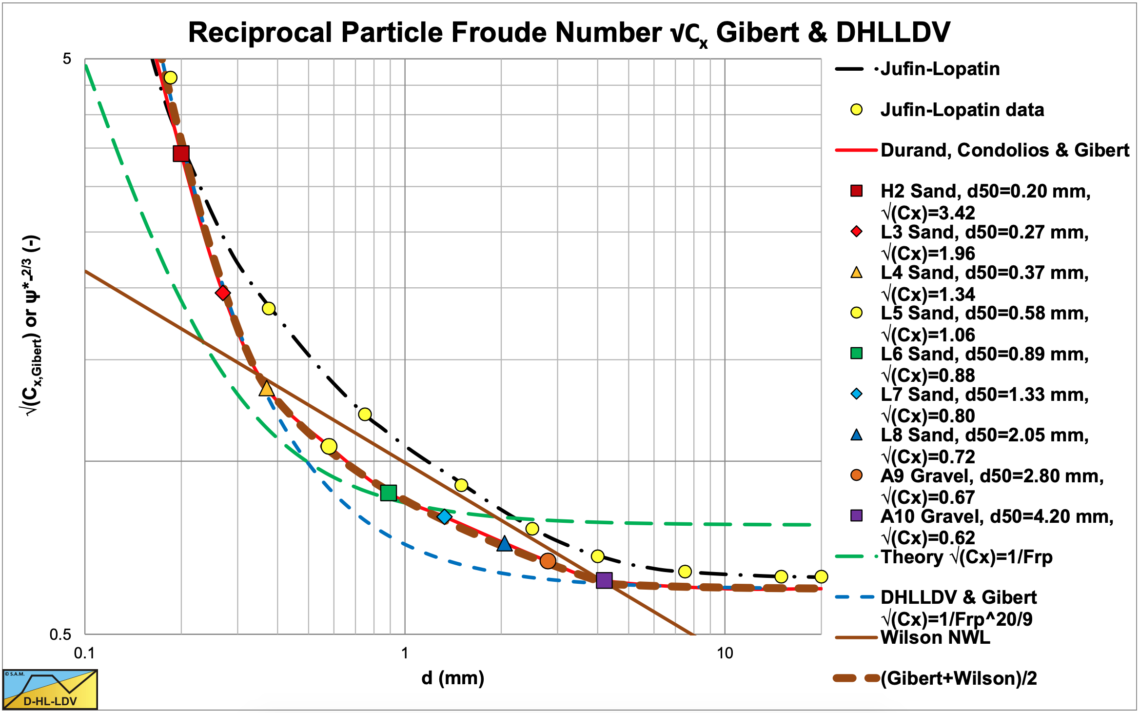
It is also possible to split the particle size distribution into n fraction and determine the weighted average particle Froude number. Gibert (1960) published a graph with values for the particle Froude number that matches the findings of Durand & Condolios (1952). Figure 6.4-20 shows these published values. If one uses the values of Gibert (1960), the whole discussion about whether the C_D or the C_x value should be used can be omitted. Analyzing this figure however, shows that a very good approximation of the table values can be achieved by using the particle Froude number to the power 20/9 instead of the power 1, assuming that the terminal settling velocity v_t is determined correctly for the solids considered (Stokes, Budryck, Rittinger or Zanke).

Figure 6.4-20 shows the original data points, the theoretical reciprocal particle Froude numbers using the Zanke (1952) equation for the terminal settling velocity of sand particles and the curve using a power of 20/9. Only for large particles there may be a small difference between the original data and the theoretical curve applying the power of 20/9.

The final equation of Durand & Condolios (1952) and later Gibert (1960) for the pressure losses now becomes:

\[\ \Delta \mathrm{p}_{\mathrm{m}}=\Delta \mathrm{p}_{\mathrm{l}} \cdot\left(1+\Phi \cdot \mathrm{C}_{\mathrm{vt}}\right)\]

With the use of the PSD modified particle Froude number:

\[\ \Phi=\frac{\mathrm{i}_{\mathrm{m}}-\mathrm{i}_{\mathrm{l}}}{\mathrm{i}_{\mathrm{l}} \cdot \mathrm{C}_{\mathrm{vt}}}=\frac{\Delta \mathrm{p}_{\mathrm{m}}-\Delta \mathrm{p}_{\mathrm{l}}}{\Delta \mathrm{p}_{\mathrm{l}} \cdot \mathrm{C}_{\mathrm{vt}}}=\mathrm{K} \cdot \Psi^{-3 / 2}=83 \cdot\left(\frac{\mathrm{v}_{\mathrm{ls}}^{2}}{\mathrm{g} \cdot \mathrm{D}_{\mathrm{p}} \cdot \mathrm{R}_{\mathrm{sd}}} \cdot \sqrt{\mathrm{C}_{\mathrm{x}}}\right)^{-3 / 2}\]

Based on the current research and Figure 6.4-20 this can be written as:

\[\ \Phi=\mathrm{8 3} \cdot\left(\frac{\mathrm{v}_{\mathrm{l s}}^{2}}{\mathrm{g} \cdot \mathrm{D}_{\mathrm{p}} \cdot \mathrm{R}_{\mathrm{s d}}} \cdot \frac{\mathrm{1}}{\mathrm{F r}_{\mathrm{p}}^{\mathrm{2 0/9}}}\right)^{-\mathrm{3 / 2}}\]

Figure 9.5-1: Modified reciprocal particle Froude number, determined experimentally for various sorts of sand and gravel by Durand & Condolios (1952) and Gibert (1960).

9.5.4.2 Wilson et al. Heterogeneous

Wilson (1997) has defined a stratification ratio or relative solids effect, which tells which fraction of the particles is in suspension and which part is in the fixed or moving bed, supported by granular contact. Wilson (1997) gives the following general equation for the head losses in hydraulic transport, where μ_sf equals the friction factor of a sliding bed, which he has determined to be μ_sf=0.44. For the 50% case at line speed v₅₀ this gives:

\[\ \mathrm{E}_{\mathrm{r h g}}=\mathrm{R}=\frac{\mathrm{i}_{\mathrm{m}}-\mathrm{i}_{\mathrm{l}}}{\mathrm{R}_{\mathrm{s d}} \cdot \mathrm{C}_{\mathrm{v t}}}=\frac{\Delta \mathrm{p}_{\mathrm{m}}-\Delta \mathrm{p}_{\mathrm{l}}}{\rho_{\mathrm{l}} \cdot \mathrm{g} \cdot \Delta \mathrm{L} \cdot \mathrm{R}_{\mathrm{s d}} \cdot \mathrm{C}_{\mathrm{v t}}}=\frac{\mu_{\mathrm{s f}}}{\mathrm{2}} \cdot\left(\frac{\mathrm{v}_{\mathrm{5 0}}}{\mathrm{v}_{\mathrm{l s}}}\right)^{\mathrm{M}}\]

When the line speed v_ls equals the v₅₀, the stratification ratio is 0.22 or half the sliding friction coefficient μsf. This can be written in terms of pressures instead of hydraulic gradient as:

\[\ \Delta \mathrm{p}_{\mathrm{m}}=\Delta \mathrm{p}_{\mathrm{l}}+\frac{\mu_{\mathrm{s f}}}{\mathrm{2}} \cdot \rho_{\mathrm{l}} \cdot \mathrm{g} \cdot \Delta \mathrm{L} \cdot\left(\frac{\mathrm{v}_{\mathrm{5 0}}}{\mathrm{v}_{\mathrm{l s}}}\right)^{\mathrm{M}} \cdot \mathrm{R}_{\mathrm{s d}} \cdot \mathrm{C}_{\mathrm{v t}}\]

Notice that here the solids effect does not depend on the carrier liquid pressure or hydraulic gradient as it does in equation (6.4-9). This equation can be written in the more generic form, matching the notations of the other theories:

\[\ \Delta \mathrm{p}_{\mathrm{m}}=\Delta \mathrm{p}_{\mathrm{l}} \cdot \left(\mathrm{1 + \frac { \mu _ { \mathrm { s f } } \cdot \mathrm { g } \cdot \mathrm { R } _ { \mathrm { s d } } \cdot \mathrm { D } _ { \mathrm { p } } } { \lambda _ { \mathrm { l } } } \cdot ( \mathrm { v } _ { \mathrm { 5 0 } } ) ^ { \mathrm { M } } \cdot ( \frac { \mathrm { 1 } } { \mathrm { v } _ { \mathrm { l s } } } ) ^ { 2 + \mathrm { M } } \cdot \mathrm { C } _ { \mathrm { v t } }}\right)\]

For the line speed, where 50% of the particles are in granular contact, v₅₀, Wilson gives the following equation:

\[\ \mathrm{v}_{50}=\mathrm{w}_{50} \cdot \sqrt{\frac{\mathrm{8}}{\lambda_{\mathrm{l}}}} \cdot \cosh \left(\frac{\mathrm{6 0} \cdot \mathrm{d}_{50}}{\mathrm{D}_{\mathrm{p}}}\right)\]

When the power M equals 1, equation (6.20-53) has the same form as the equation of Durand & Condolios (1952), Gibert (1960), Fuhrboter (1961), Jufin Lopatin (1966) and Newitt et al. (1955). The power M depends on the grading of the sand and can be determined by:

\[\ \mathrm{M=\left(0.25+13 \cdot \sigma^{2}\right)^{-1 / 2}}\]

The variance σ of the PSD (Particle Size Distribution), can be determined by some ratio between the v₅₀ and the v₈₅:

\[\ \sigma=\log \left(\frac{\mathrm{v}_{85}}{\mathrm{v}_{50}}\right)=\log \left(\frac{\mathrm{w}_{85} \cdot \sqrt{\frac{8}{\lambda_{\mathrm{l}}}} \cdot \cosh \left(\frac{60 \cdot \mathrm{d}_{85}}{\mathrm{D}_{\mathrm{p}}}\right)} { \mathrm{w_{50}} \cdot \sqrt{\frac{\mathrm{8}}{\lambda_{\mathrm{l}}} \cdot \cosh \left(\frac{60 \cdot \mathrm{d}_{50}}{\mathrm{D}_{\mathrm{p}}}\right)}}\right)\]

The terminal settling velocity related parameter w, the particle associated velocity, can be determined by:

\[\ \mathrm{w}=\mathrm{0 .9} \cdot \mathrm{v}_{\mathrm{t}}+\mathrm{2 .7} \cdot\left(\mathrm{R}_{\mathrm{s d}} \cdot \mathrm{g} \cdot v_{\mathrm{l}}\right)^{1 / 3}\]

It seems this equation mixes the homogeneous and heterogeneous regimes. For very small particles the second term gives a constant particle associated velocity, which matches homogeneous behavior at operational line speeds. Since the homogeneous behavior does not depend on the particle size, this gives a constant or asymptotic particle associated velocity. The model of Wilson can be simplified with some fit functions, according to:

\[\ \mathrm{v}_{\mathrm{5 0}} \approx \mathrm{3 .9 3} \cdot\left(\frac{\mathrm{d}_{\mathrm{5 0}}}{\mathrm{0 .0 0 1}}\right)^{\mathrm{0 .3 5}} \cdot\left(\frac{\mathrm{R}_{\mathrm{s d}}}{\mathrm{1 .6 5}}\right)^{\mathrm{0 . 4 5}} \cdot\left(\frac{v_{\mathrm{l}, \mathrm{a c t u a l}}}{v_{\mathrm{w}, \mathrm{2 0}}}\right)^{-\mathrm{0 . 2 5}}\]

In which the particle diameter d₅₀ is in m and the resulting v₅₀ in m/s. The third term on the right had side is the relative viscosity, the actual liquid viscosity divided by the viscosity of water at 20 degrees Centigrade. In normal dredging practice this term is about unity and can be neglected. The factor 1.65 is based on sand in clear water.

The simplified exponent M is given by the approximation:

\[\ \mathrm{M} \approx\left(\ln \left(\frac{\mathrm{d}_{85}}{\mathrm{d}_{50}}\right)\right)^{-1}\]

Later the simplified equation for the v50 has been adjusted for particles with diameters from 0.2 mm to 0.5 mm with a factor, Sellgren et al. (2016) and Miedema (June 2016):

\[\ \mathrm{f=\frac{d_{h}-0.0002}{0.0005-0.0002} \quad\text{ or }\quad f=\frac{d_{h}-0.0001}{0.0004-0.0001}}\]

The second equation however gives a more reasonable fit for particles between 0.1 mm and 0.4 mm. An even better simplification of the v50 is achieved with the following equation (DHLLDV simplified, the dash-dot green line):

\[\ \mathrm{v}_{\mathrm{5 0}} \approx \mathrm{3} \cdot\left(\frac{\mathrm{d}_{\mathrm{5 0}}}{\mathrm{0 .0 0 0 5}}\right)^{\mathrm{0 . 4 5}} \cdot\left(\frac{\mathrm{R}_{\mathrm{s d}}}{\mathrm{1 .6 5}}\right)^{\mathrm{0 . 4 5}} \cdot\left(\frac{v_{\mathrm{l}, \mathrm{a c t u a l}}}{v_{\mathrm{w}, \mathrm{2 0}}}\right)^{-\mathrm{0 . 2 5}} \cdot\left(\frac{\mathrm{D}_{\mathrm{p}}}{\mathrm{0 .1 5 2 4}}\right)^{\mathrm{0 . 0 9 2}}\]

A better approach of the v₅₀ however is the following equation, based on the DHLLDV Framework:

\[\ \mathrm{v}_{\mathrm{5 0}} \approx \mathrm{3 .4} \cdot\left(\frac{\mathrm{v}_{\mathrm{t}}}{\sqrt{\mathrm{g} \cdot \mathrm{d}}}\right)^{\mathrm{1 .9 6}} \cdot\left(\frac{\mathrm{D}_{\mathrm{p}}}{\mathrm{0 .1 5 2 4}}\right)^{\mathrm{0 . 0 9 2}} \cdot\left(\frac{\mathrm{R}_{\mathrm{s d}}}{\mathrm{1 .6 5}}\right)^{-\mathrm{0 . 0 9 2}} \cdot\left(\frac{v_{\mathrm{l}, \mathrm{a c t u a l}}}{v_{\mathrm{w}, \mathrm{2 0}}}\right)^{\mathrm{0 . 2 7}}\]

Figure 9.5-2: The different v₅₀ methods.

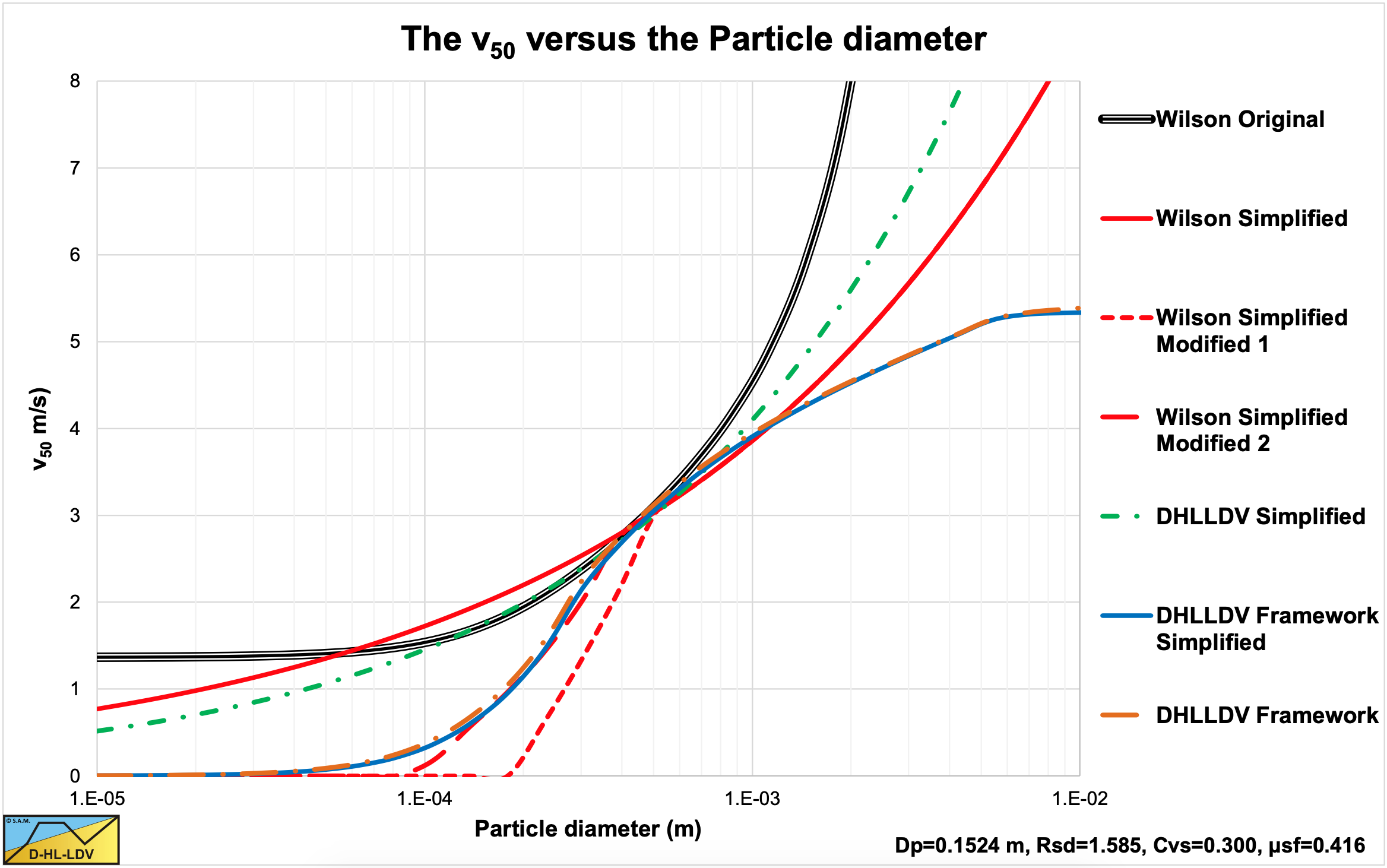
Figure 9.5-2 shows the different v₅₀ methods. The thick black solid line shows the original v₅₀ method of Wilson et al. (1992). For very small particles and very large particles this method overestimates the v₅₀. For very small particles because of homogeneous transport under operational conditions, for very large particles because of the occurrence of a sliding bed. For particles in the range of d=0.3 mm to d=0.8 mm the estimated v₅₀ values seem to be reasonable. The thin red solid line shows the simplified equation, which is close to the original in the range of d=0.1 mm to d=1 mm, although the fit could be much better. The dash-dot green line shows the result of the DHLLDV simplified equation, giving a much closer fit to the original Wilson et al. (1992) method. Later the simplified equation (6.20-58) was adjusted with a factor to get rid of the overestimation for small particles with equation (6.20-75). Both possibilities are drawn in Figure 9.5-2. The first equation is the red dashed line and the second equation the dash-dot red line. Still the equations include the influence of the homogeneous regime for very small particles and the sliding bed regime for very large particles. Using a factor to compensate for the homogeneous overestimation is understandable, but not based on physics. Based on the DHLLDV Framework the v₅₀ can also be determined. Although this Framework is more complicated, the line speed where the heterogeneous hydraulic gradient matches the hydraulic gradient of a sliding bed with 50% of the sliding friction coefficient is possible. This is the light brown dash-dot line in the graph. For medium sands this line matches both the original Wilson et al. (1992) method and the simplified equations. It also matches the use of the factor (2^nd) to get rid of the overestimation for very small particles. For very large particles this gives much smaller v₅₀ values, since the formulation of the heterogeneous regime of the DHLLDV Framework is not influenced by the sliding bed regime. Equation (9.5-31) is a simplification of the DHLLDV Framework (the solid blue line), matching the full Framework very accurate. For the Wilson et al. (1992) model for graded sands equation (9.5-31) will be used for the determination of the v₅₀.

It should be mentioned that the original Wilson et al. (1992) method and the simplified equation are not consistent with regard to the viscosity. With an increasing viscosity, the original method will give an increasing v₅₀, while the simplified equation gives a decreasing v₅₀. This is caused by the second term in equation (9.5-26) for the particle associated velocity, which increases with increasing viscosity, while the settling velocity will decrease. The correct behavior is a decreasing v₅₀ with increasing viscosity, due to the decrease of the settling velocity. In equation (9.5-31) the term containing the settling velocity decreases much faster than the increase of the term with the viscosity, giving a decrease of the v₅₀ with increasing viscosity, similar to the simplified equations.

9.5.4.3 The Modified 4 Component Model

The original 4 component model (4CM) (Sellgren & Wilson (2007)) assumes that each coarser fraction is moving in a carrier liquid containing all finer fractions. So, the coarsest stratified fraction is moving in a carrier liquid containing the homogeneous, pseudo homogeneous and heterogeneous fractions, increasing the carrier liquid density and thus decreasing the relative submerged density and the settling velocity. Only the homogeneous fraction influences the viscosity of the carrier liquid. The original 4CM model up to Sellgren et al. (2014) contains some errors regarding the determination of the different carrier liquid densities, which have been corrected, after Miedema & Ramsdell (2015) discovered this, in Sellgren et al. (2016) as also mentioned in Miedema (June 2016). Still in Sellgren et al. (2016) there is an error in equation 13 for the fully stratified flow. The factor 0.55 should be to the power 0.25. In the original article, Sellgren et al. (2014) this was still correct. The original model for fully stratified flow is, using the sliding friction factor of 0.44:

\[\ \begin{array}{left}\mathrm{i}_{\mathrm{m}}=\mathrm{i}_{\mathrm{l}}+\mathrm{B}^{\prime} \cdot \mathrm{R}_{\mathrm{s} \mathrm{d}} \cdot \mathrm{C}_{\mathrm{v} \mathrm{t}} \cdot\left(\frac{\mathrm{0 . 5 5} \cdot \mathrm{v}_{\mathrm{s m}}}{\mathrm{v}_{\mathrm{l s}}}\right)^{\mathrm{0 . 2 5}}\\
\mathrm{i}_{\mathrm{m}}=\mathrm{i}_{\mathrm{l}}+\mathrm{B}^{\prime} \cdot \mathrm{R}_{\mathrm{s d}} \cdot \mathrm{C}_{\mathrm{v t}} \cdot \mathrm{2} \cdot \mu_{\mathrm{s f}} \cdot\left(\frac{\mathrm{v}_{\mathrm{s m}}}{\mathrm{v}_{\mathrm{l} \mathrm{s}}}\right)^{\mathrm{0 . 2 5}}\end{array}\]

Wilson et al. (1992) used a sliding friction factor of 0.44 in the derivation of the 2-layer model. Based on his hydrostatic approach the factor 2 is valid for plug flow if the spatial volumetric concentration equals the bed concentration. A more general notation can be given by, based on the spatial concentration (note the factor 2 is omitted):

\[\ \mathrm{i}_{\mathrm{m}}=\mathrm{i}_{\mathrm{l}}+\mathrm{B} \cdot \mathrm{R}_{\mathrm{s} \mathrm{d}} \cdot \mathrm{C}_{\mathrm{v s}} \cdot \mu_{\mathrm{s f}} \cdot\left(\frac{\mathrm{v}_{\mathrm{s m}}}{\mathrm{v}_{\mathrm{l} \mathrm{s}}}\right)^{\mathrm{0 . 2 5}}\]

With the factor B in the hydrostatic normal stress approach equals (with β the bed angle with the vertical):

\[\ \mathrm{B}=\frac{2 \cdot(\sin (\beta)-\beta \cdot \cos (\beta))}{(\beta-\sin (\beta) \cdot \cos (\beta))}\]

The factor B is included, because with β=π the term describes plug flow, B=2. For β<π the factor B decreases with β, β=π/2 gives B=1.3 and β=0 gives B=1. So, for low concentrations and small fully stratified fractions a value of B=1 should be chosen, which matches the later choice of Wilson for a B’=0.5 (originally he mentioned B’ is close to unity). Sellgren et al. (2014) use B’=0.25 (B=0.5), while in the reprint of the article Sellgren et al. (2016) they use B’=0.35 (B=0.7). The weight approach of Miedema & Ramsdell (2014) also uses B=1. To convert the equation from spatial volumetric concentration to delivered volumetric concentration, the slip ratio ξ_vsm at the line speed v_sm should be known, giving:

\[\ \mathrm{i}_{\mathrm{m}}=\mathrm{i}_{\mathrm{l}}+\mathrm{B} \cdot \mathrm{R}_{\mathrm{s} \mathrm{d}} \cdot \frac{\mathrm{C}_{\mathrm{v t}}}{\mathrm{1}-\xi_{\mathrm{v} \mathrm{s} \mathrm{m}}} \cdot \mu_{\mathrm{s f}} \cdot\left(\frac{\mathrm{v}_{\mathrm{s m}}}{\mathrm{v}_{\mathrm{l s}}}\right)^{\mathrm{0 . 2 5}}\]

The effect of the decreasing slip ratio with increasing line speed is taken into account with the term (v_sm/v_ls)^0.25. The slip ratio can be estimated by the following empirical equation, based on the 2-layer model with sheet flow added (so 3LM), Miedema (June 2016):

\[\ \begin{array}{left}{\mathrm{C}}_{\mathrm{v r}}=\frac{\mathrm{C}_{\mathrm{v t}}}{\mathrm{C}_{\mathrm{v} \mathrm{b}}} \quad\text{ and }\quad \alpha=\mathrm{0 .5 8} \cdot \mathrm{C}_{\mathrm{v r}}^{-\mathrm{0 . 4 2}} \quad\text{ and }\quad\frac{\mathrm{B}}{1-\xi_{\mathrm{v s m}}}=\mathrm{C}_{\mathrm{v r}}^{-\mathrm{0 . 5}}\\ \xi=\left(1-\mathrm{C}_{\mathrm{v r}}\right) \cdot \mathrm{e}^{\left(-\left(0.83+\frac{\mu_{\mathrm{sf}}}{4}+\left(\mathrm{c}_{\mathrm{vr}}-\mathrm{0 . 5 - 0 . 0 7 5 . 0}\right)^{2}+0.025 \cdot \mathrm{D}_{\mathrm{p}}\right) \cdot \mathrm{D}_{\mathrm{p}}^{0.025} \cdot\left(\frac{v_{\mathrm{ls}}}{v_{\mathrm{sm}}}\right)^{\alpha} \cdot \mathrm{C}_{\mathrm{vr}}^{0.65}\right.}\end{array}\]

This way the slip ratio is incorporated in the model and B’ depends on this slip ratio. A better approximation of the hydraulic gradient is, using the line speed dependent slip ratio (B=1 weight approach, B=equation (9.5-34) hydrostatic approach):

\[\ \mathrm{i}_{\mathrm{m}}=\mathrm{i}_{\mathrm{l}}+\mathrm{B} \cdot \mathrm{R}_{\mathrm{s d}} \cdot \frac{\mathrm{C}_{\mathrm{v t}}}{\mathrm{1}-\xi} \cdot \mu_{\mathrm{s f}}\]

The maximum of course is plug flow, so if plug flow is reached, the hydrostatic Wilson approach gives as an upper limit:

\[\ \mathrm{i}_{\mathrm{m}}=\mathrm{i}_{\mathrm{l}}+\mathrm{2} \cdot \mathrm{R}_{\mathrm{s} \mathrm{d}} \cdot \mathrm{C}_{\mathrm{v} \mathrm{b}} \cdot \boldsymbol{\mu}_{\mathrm{s f}}\]

The weight approach of Miedema & Ramsdell (2014) gives for the plug flow upper limit (this follows from substituting equation (7.4-93) in equation (9.5-37) at v_ls=0):

\[\ \mathrm{i}_{\mathrm{m}}=\mathrm{i}_{\mathrm{l}}+\mathrm{R}_{\mathrm{s d}} \cdot \mathrm{C}_{\mathrm{v b}} \cdot \boldsymbol{\mu}_{\mathrm{s f}}\]

In the 4CM each coarser fraction floats in all finer fractions. So, the buoyancy of coarser fractions increases with increasing finer fractions. This seems strange since a bed is a bed, including all fractions in the bed. The small fractions in the bed do not make the coarse fractions lighter. So, in the modified 4CM, only the homogeneous fraction is assumed to influence the density and the viscosity of the carrier liquid (see the adjusted liquid properties). This gives for the relative density S_f of the homogeneous mixture of particles with d<0.000040 m:

\[\ \mathrm{S_{f}=\frac{\rho_{f}}{\rho_{l}}=1+\frac{X_{f} \cdot C_{v s} \cdot R_{s d}}{1-C_{v s} \cdot\left(1-X_{f}\right)}}\]

The hydraulic gradient of the homogeneous flow regime i_f is now:

\[\ \mathrm{i}_{\mathrm{f}}=\frac{\rho_{\mathrm{f}}}{\rho_{\mathrm{l}}} \cdot \frac{\lambda_{\mathrm{f}} \cdot \mathrm{v}_{\mathrm{l s}}^{2}}{2 \cdot \mathrm{g} \cdot \mathrm{D}_{\mathrm{p}}}=\mathrm{S}_{\mathrm{f}} \cdot \frac{\lambda_{\mathrm{f}} \cdot \mathrm{v}_{\mathrm{ls}}^{2}}{2 \cdot \mathrm{g} \cdot \mathrm{D}_{\mathrm{p}}}=\frac{\rho_{\mathrm{f}}}{\rho_{\mathrm{l}}} \cdot \mathrm{i}_{\mathrm{l}}=\mathrm{S}_{\mathrm{f}} \cdot \mathrm{i}_{\mathrm{l}}\]

The difference with pure carrier liquid is the Darcy Weisbach friction factor and the relative density S_f of the resulting homogeneous fluid. For small homogeneous fractions, the Darcy Weisbach friction factor will not differ much from the factor determined for the carrier liquid. So, the main difference is the use of the relative density S_f>1 instead of 1. The resulting hydraulic gradient of the modified 4 component model is now:

\[\ \mathrm{i}_{\mathrm{m}}=\frac{\rho_{\mathrm{f}}}{\rho_{\mathrm{l}}} \cdot \mathrm{i}_{\mathrm{f}}+\frac{\rho_{\mathrm{f}}}{\rho_{\mathrm{l}}} \cdot \mathrm{C}_{\mathrm{v t}} \cdot \mathrm{R}_{\mathrm{s} \mathrm{d}, \mathrm{f}} \cdot\left(\mathrm{A} \cdot \mathrm{X}_{\mathrm{p h}} \cdot \mathrm{i}_{\mathrm{f}}+\mathrm{X}_{\mathrm{h}} \cdot \frac{\mu_{\mathrm{s} \mathrm{f}}}{\mathrm{2}} \cdot\left(\frac{\mathrm{v}_{\mathrm{5} 0, \mathrm{f}}}{\mathrm{v}_{\mathrm{l s}}}\right)^{\mathrm{M}}+\mathrm{B} \cdot \frac{\mathrm{X}_{\mathrm{s}}}{1-\xi_{\mathrm{v} \mathrm{s} \mathrm{m}}} \cdot \mu_{\mathrm{s} \mathrm{f}} \cdot\left(\frac{\mathrm{v}_{\mathrm{s} \mathrm{m}, \mathrm{f}}}{\mathrm{v}_{\mathrm{l} \mathrm{s}}}\right)^{0.25}\right)\]

The factor A<1 is included because often the excess hydraulic gradient is smaller than the ELM would give, because of near wall lift. A value of A=0.5-0.6 is found to be reasonable. For the factor B a value of 1 is applied. Sellgren et al. (2016) give a smaller value of about 0.7, which is difficult to compare, since they do not use the slip ratio. The power M in the 4CM model is assumed to be 1. The v_50,f and v_sm,f values are determined based on the adjusted carrier liquid. Physically this is a 3-layer model, with the homogeneous fraction forming an adjusted carrier liquid, the fully stratified fraction forming a sliding bed, the heterogeneous fraction on top of the sliding bed and the pseudo homogeneous fraction at the top of the pipe. For small concentrations, however, there is not much difference with the original 4CM model, but for large concentrations there may be a difference depending on the PSD. The d₅₀ of the heterogeneous fraction of the 4CM should be determined according to:

\[\ \mathrm{d}_{\mathrm{5 0}, \mathrm{4 C M}}=\sqrt{\mathrm{0 .0 0 0 2} \cdot \mathrm{0 .0 1 5} \cdot \mathrm{D}_{\mathrm{p}}}\]

Or by constructing the PSD of the heterogeneous fraction and reading the d₅₀ from the resulting graph. Both methods give about the same d₅₀.

9.5.4.4 Wilson 4 Regime Model

The adjustment of the properties of the carrier liquid is similar to the other models as described in this chapter. The determination of the stratified flow regime is similar tot he fully stratified flow in the 4CM, but now with 100% of the particles in the stratified flow regime. The determination of the heterogeneous flow regime is similar to the original Wilson heterogeneous flow regime. The new element in this model is the transition of the Wilson heterogeneous flow regime tot he high speed homogeneous flow regime. Wilson defined a stratification ratio determining the fraction of the solids being in the stratified flow. This stratification ratio is:

\[\ \mathrm{R}=\frac{1}{2} \cdot\left(\frac{\mathrm{v}_{50}}{\mathrm{v}_{\mathrm{ls}}}\right)^{\mathrm{M}}\]

So if the line speed v_ls equals the v₅₀ of Wilson, 50% of the solids is stratified. This also implies that the other 50% is in suspension. The total solids effect is thus the stratification ratio R times the hydraulic gradient of a sliding bed plus (1-R) times the hydraulic gradient of homogeneous flow. This gives a smooth transition of the heterogeneous flow regime to the homogeneous flow regime, giving:

\[\ \mathrm{i}_{\mathrm{m}}-\mathrm{i}_{\mathrm{l}}=\mathrm{C}_{\mathrm{v} \mathrm{t}} \cdot \mathrm{R}_{\mathrm{s} \mathrm{d}} \cdot\left(\mu_{\mathrm{s f}} \cdot \frac{\mathrm{1}}{\mathrm{2}} \cdot\left(\frac{\mathrm{v}_{\mathrm{5} 0}}{\mathrm{v}_{\mathrm{l s}}}\right)^{\mathrm{M}}+\mathrm{A} \cdot \mathrm{i}_{\mathrm{l}} \cdot\left(\mathrm{1}-\frac{\mathrm{1}}{\mathrm{2}} \cdot\left(\frac{\mathrm{v}_{\mathrm{5} 0}}{\mathrm{v}_{\mathrm{l s}}}\right)^{\mathrm{M}}\right)\right)\]

The factor A is introduced, because from experiments it is known that the hydraulic gradient in the homogeneous flow regime is smaller than the ELM, with a reduction of A=0.5-0.6. In the above reasoning it is assumed that the two flow regimes are independent and can be summed in a linear way. In reality there will be a certain interaction, influencing the transition.

9.5.4.5 The DHLLDV Framework

The DHLLDV Framework is extensively described in Miedema (June 2016) and will not be described in detail here. The Framework combines the 5 main flow regimes, the stationary bed regime, the sliding bed regime, the heterogeneous flow regime or sliding flow regime and the homogeneous flow regime, for uniform sands and gravels and constant spatial volumetric concentrations. The result is a hydraulic gradient curve where all flow regimes may be present depending on pipe and particle diameter, concentration and line speed. Based on a Limit Deposit Velocity model of Miedema (June 2016) the slip ratio curve is constructed and based on the slip ratio curve the constant delivered concentration curve is determined. For graded sands or gravels, the PSD is divided into a number of fractions. First the liquid properties are adjusted as described in this paper. Secondly the PSD is adjusted, not containing the fines anymore. For each resulting fraction the hydraulic gradient curve is determined based on the spatial/delivered concentration of the whole PSD in order to take hindered settling into account in a correct way. The resulting hydraulic gradient curves are multiplied with the corresponding fraction and added up. The result is a hydraulic gradient curve for the whole PSD.

9.5.5 Example of a Graded Sand

As an example of the comparison of the 5 methods a pipe diameter of D_p=0.1524 m and a d₅₀=0.5 mm are chosen, because the models for uniform sands give very similar hydraulic gradients under operational conditions (line speeds). The different v₅₀ equations also give about the same v₅₀. This way only the grading of the PSD may be the reason of differences.

Figure 9.5-3: The hydraulic gradient curves of the fractions and the resulting hydraulic gradient curve.

Figure 9.5-4: The PSD of the sand considered, D_p=0.1524 m.

Figure 9.5-5: The resulting hydraulic gradient curves, D_p=0.1524 m.

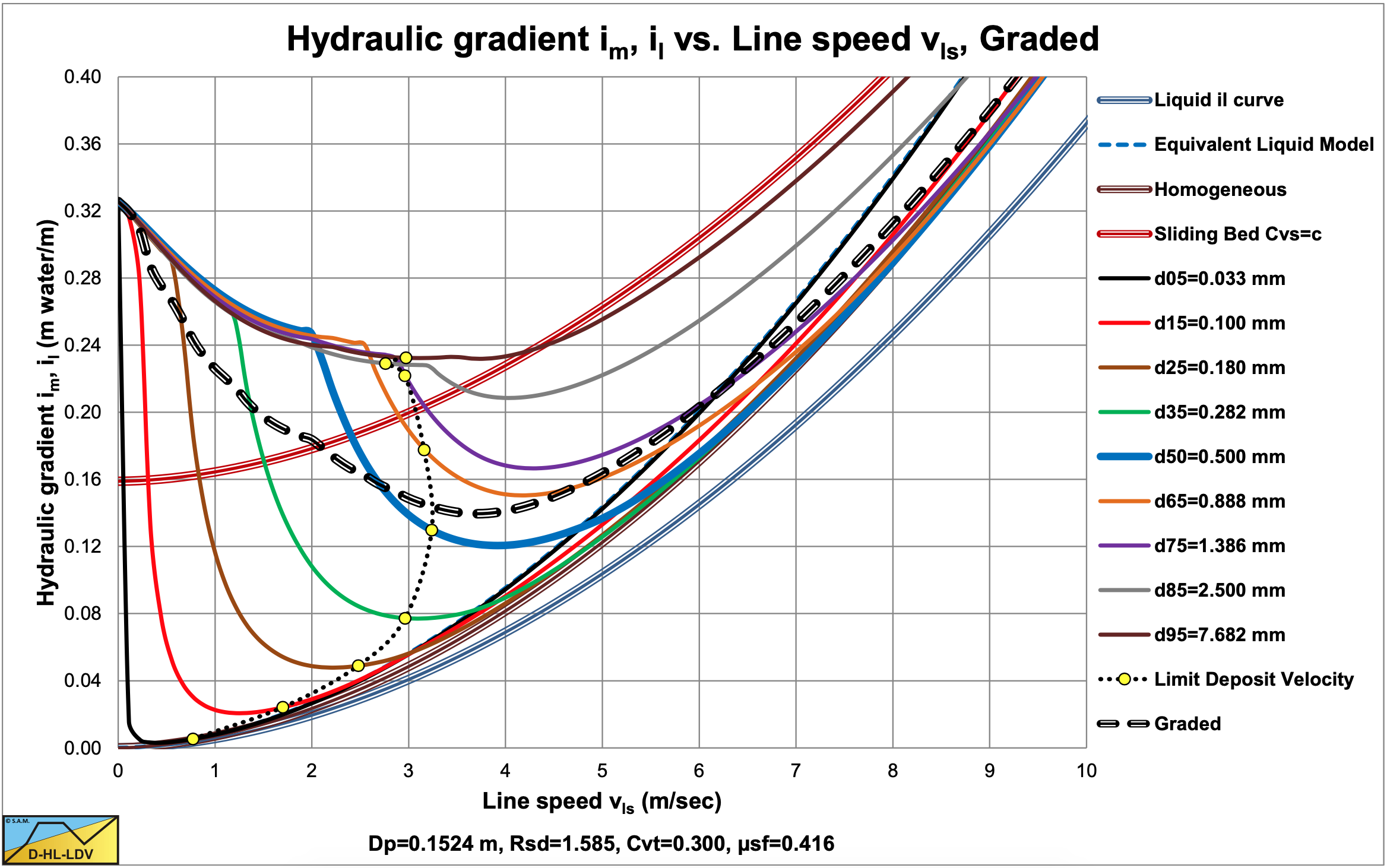
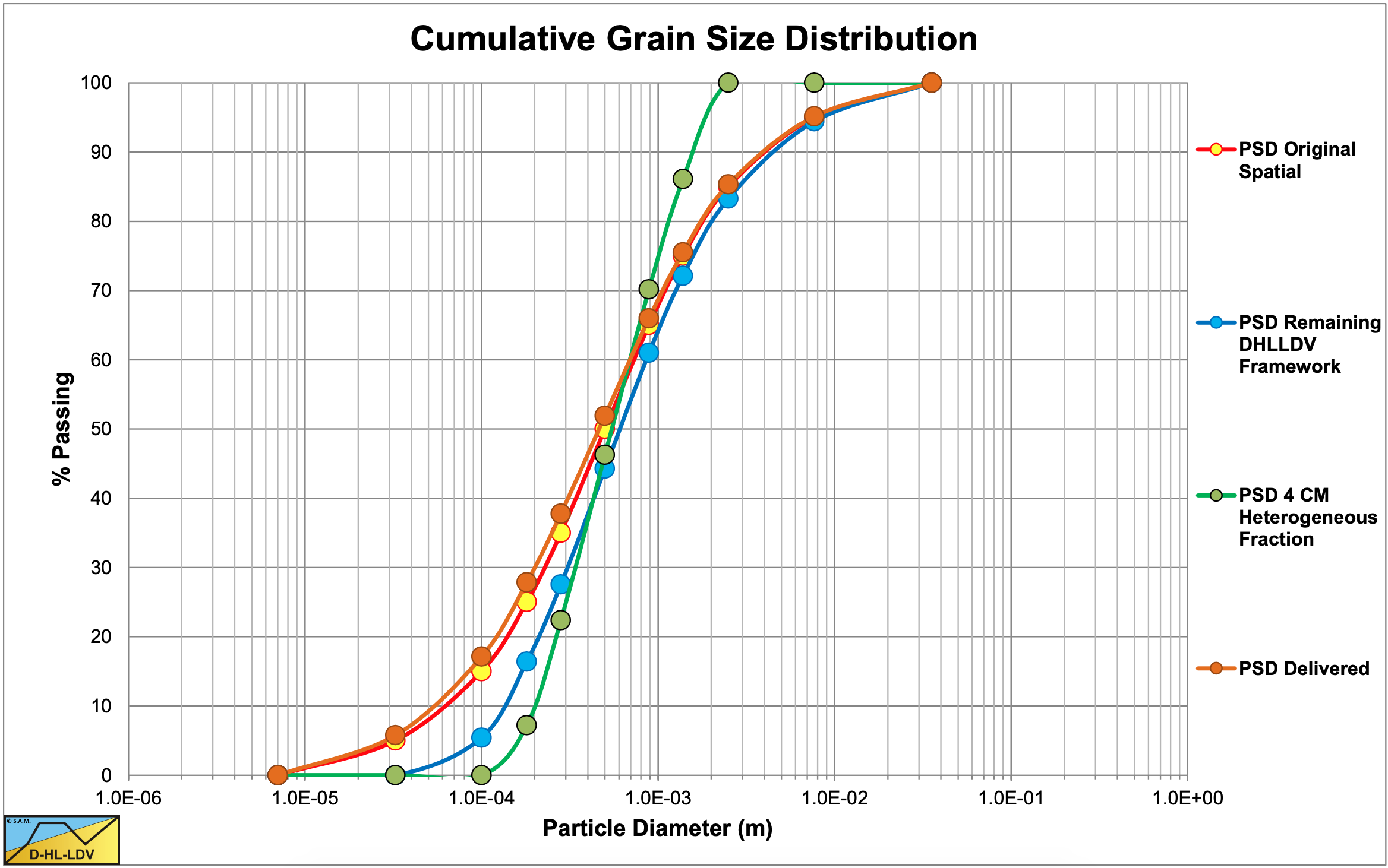
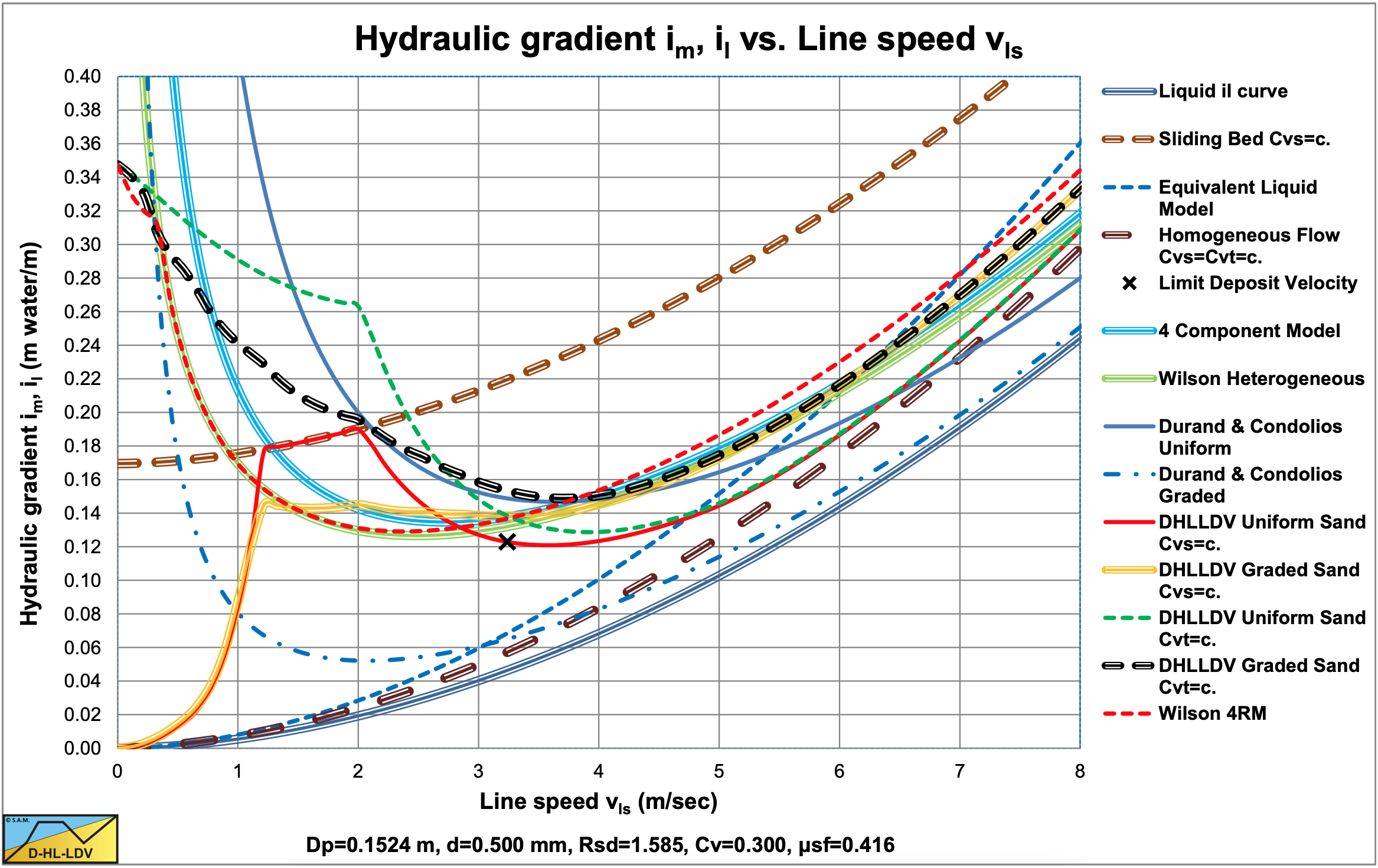
Figure 9.5-3 shows the hydraulic gradient curves of 9 fractions and the resulting hydraulic gradient curve for the DHLLDV Framework. The PSD given in Figure 9.5-4 is a very broad graded PSD in order to emphasize the effect of grading. This figure also shows the PSD corrected for the fines of the DHLLDV Framework and the heterogeneous PSD as used in the 4CM model. The graph also shows the delivered PSD which is slightly finer than the spatial PSD.

Figure 9.5-6: The resulting relative excess hydraulic gradient curves, also named the stratification ratio, D_p=0.1524 m.

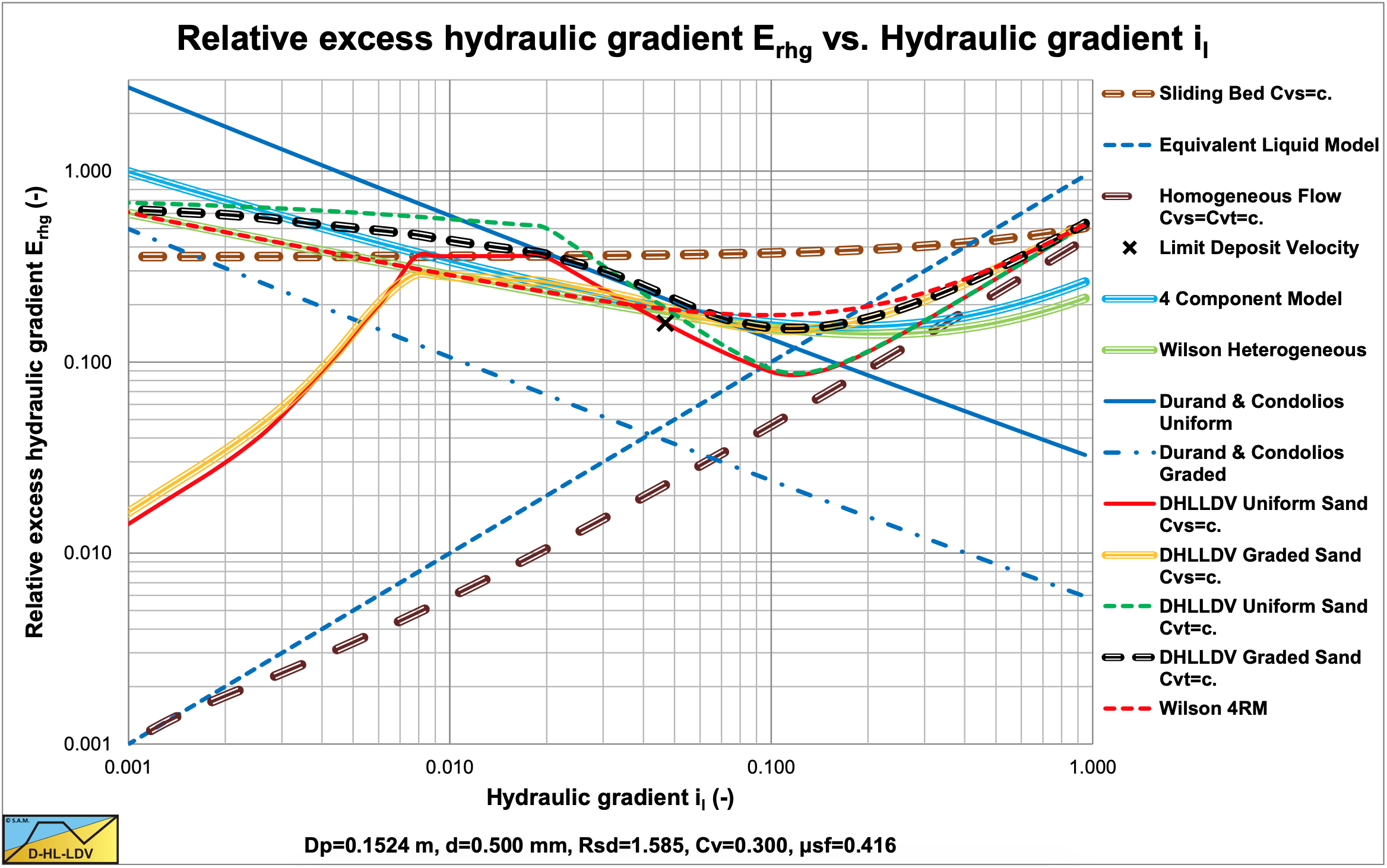
Figure 9.5-3 shows that for small line speeds the resulting hydraulic gradient (the thick dashed black line) is smaller than the corresponding hydraulic gradient of the uniform sand (the thick solid blue line). For larger line speeds (above about 2.6 m/s) however, the resulting hydraulic gradient is larger. This is similar to the effect of a reduced power M in the Wilson heterogeneous v₅₀ method, with a v₅₀ of about 3 m/s for all equations. Figure 9.5-5 and Figure 9.5-6 show a comparison of the 5 different methods. In Figure 9.5-6 the relative excess hydraulic gradient or stratification ratio as Wilson named it is shown, which is defined as:

\[\ \mathrm{E}_{\mathrm{r h g}}=\frac{\mathrm{i}_{\mathrm{m}}-\mathrm{i}_{\mathrm{l}}}{\mathrm{R}_{\mathrm{s d}} \cdot \mathrm{C}_{\mathrm{v t}}} \quad\text{ or }\quad \mathrm{E}_{\mathrm{r h g}}=\frac{\mathrm{i}_{\mathrm{m}}-\mathrm{i}_{\mathrm{l}}}{\mathrm{R}_{\mathrm{s d}} \cdot \mathrm{C}_{\mathrm{v s}}}\]

Figure 9.5-5 and Figure 9.5-6 also show the uniform curves for the Durand & Condolios (1952) model and the DHLLDV Framework (June 2016).

Figure 9.5-7: The behavior of the 4 components, D_p=0.1524 m.

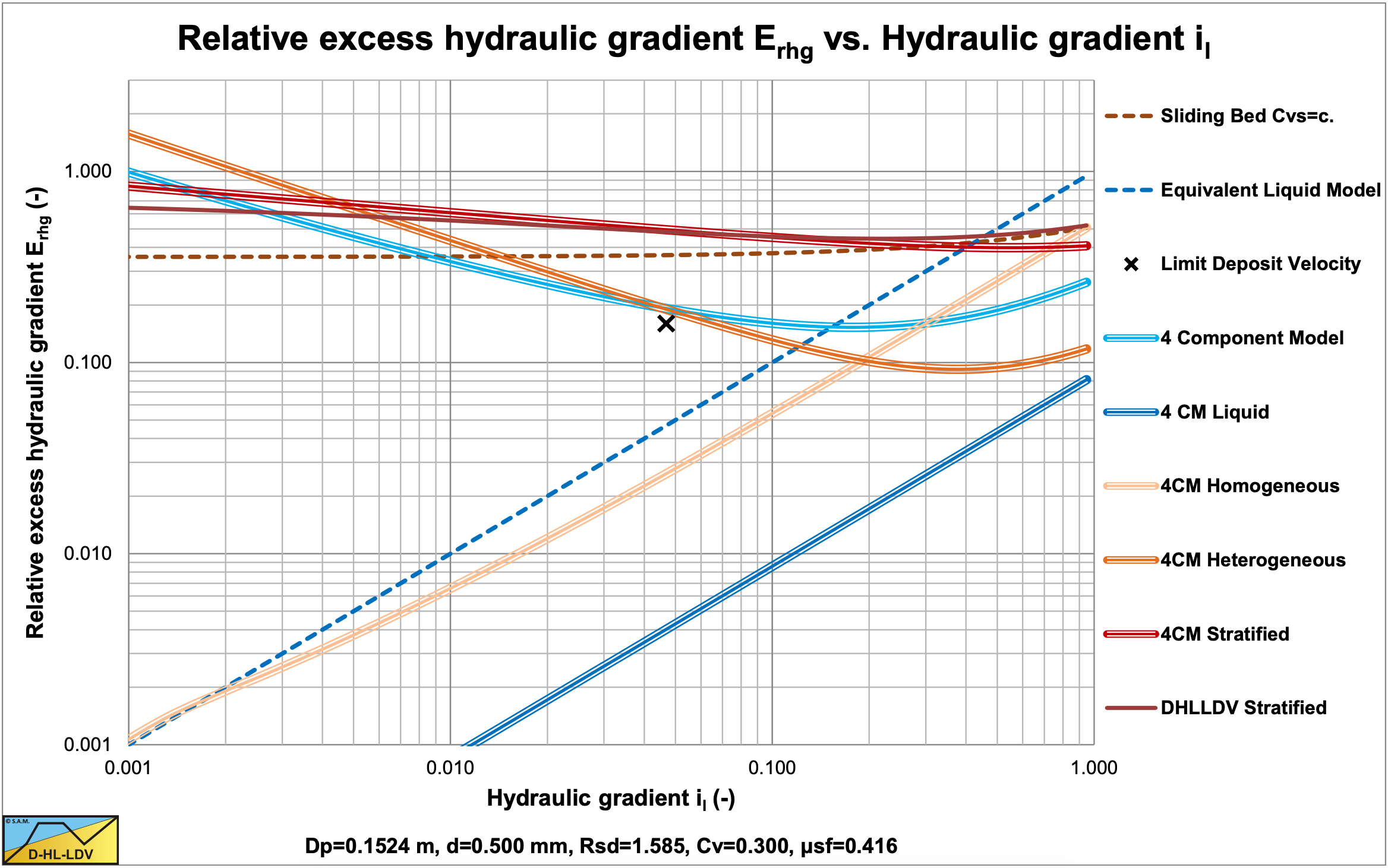
Figure 9.5-7 shows the behavior of the 4 components and the resulting 4CM curve. The graph also shows the stratified curve based on slip velocity (DHLLDV stratified). The latter is less steep as the original stratified curve with a power of 0.25. The steepness of the DHLLDV stratified curve however depends strongly on the volumetric concentration. An increasing concentration gives a decreasing steepness.

Figure 9.5-8 and Figure 9.5-9 give a close up of the hydraulic gradient and the solids effect in the operational region of line speeds. Above the LDV the hydraulic gradients are very close and within the margin of experimental scatter. The solids effect seems to give more difference, but this is because of the double logarithmic graph. The curvature of the 4CM and Wilson heterogeneous models at high hydraulic gradients is due to the adjustment of the carrier liquid properties. The Durand & Condolios model is omitted here because it is rejected. The 4CM curve location is influenced by the volumetric concentration. This curve will be higher if the concentration decreases. The other 3 models are hardly influenced by the concentration in the solids effect graph.

Figure 9.5-8: Close up of the hydraulic gradient, D_p=0.1524 m.

Figure 9.5-9: Close up of the solids effect, D_p=0.1524 m.

Figure 9.5-10: The PSD of the sand considered, D_p=0.762 m.

Figure 9.5-11: The resulting hydraulic gradient curves, D_p=0.762 m.

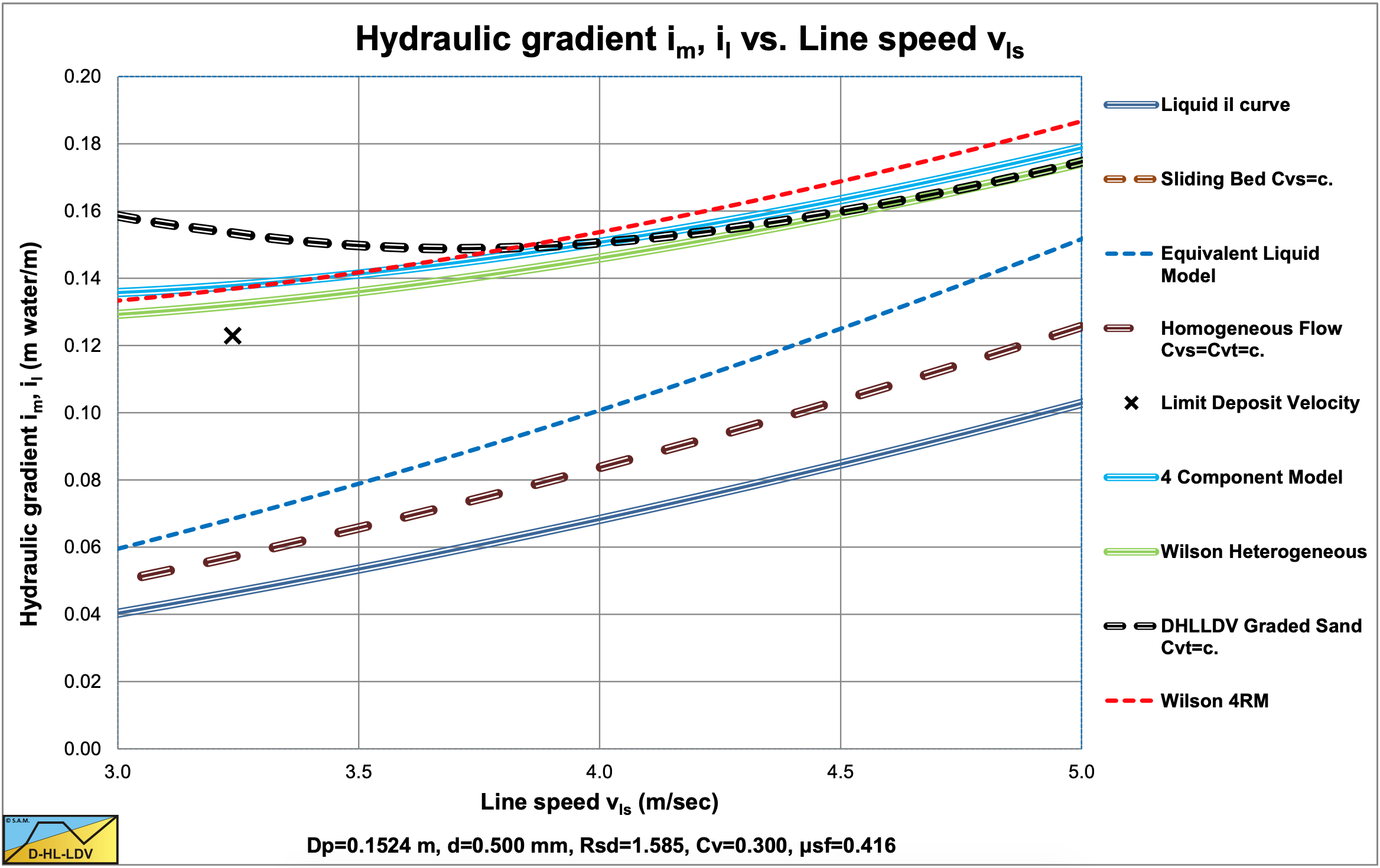
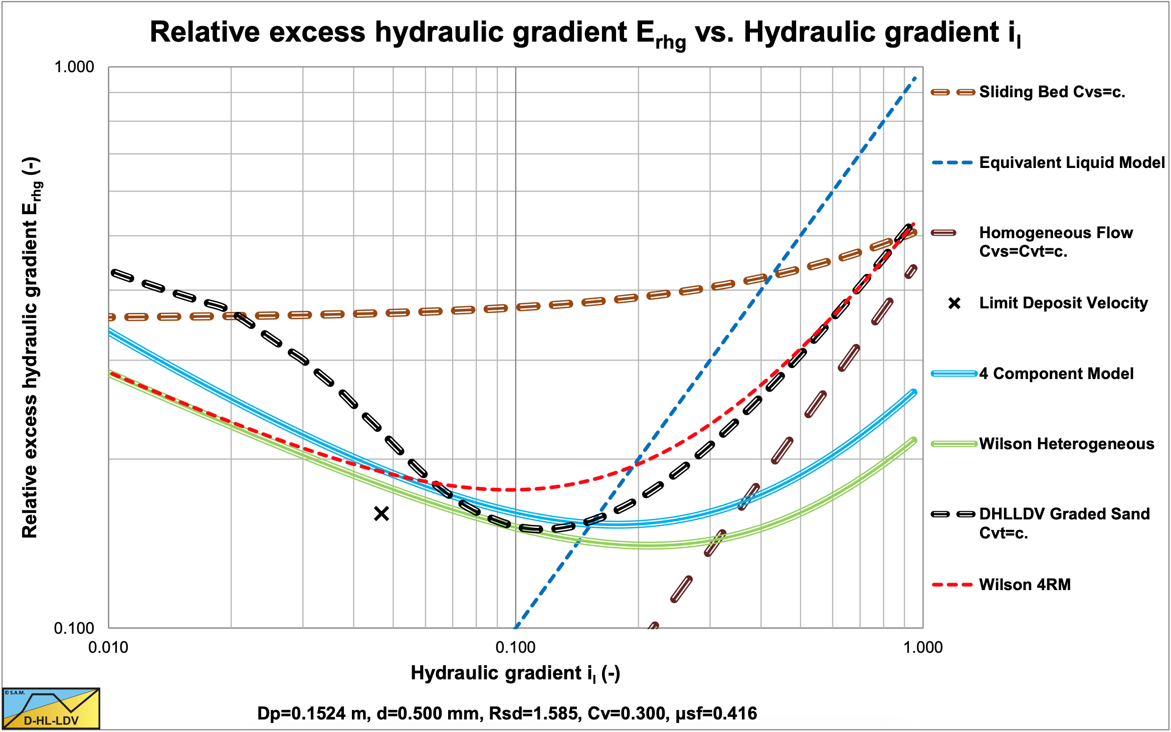
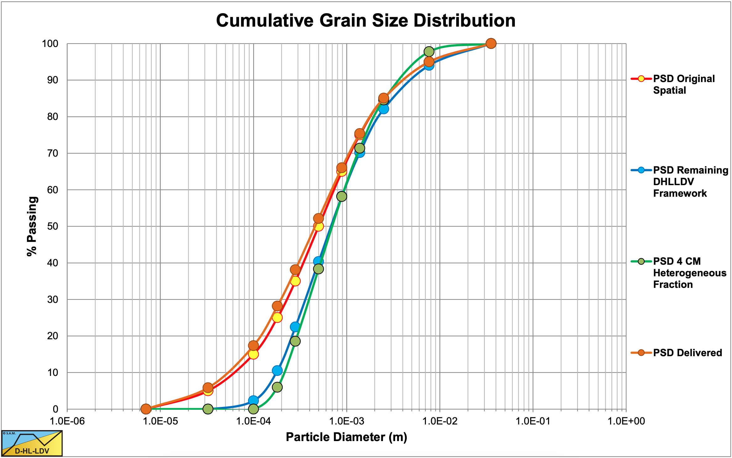
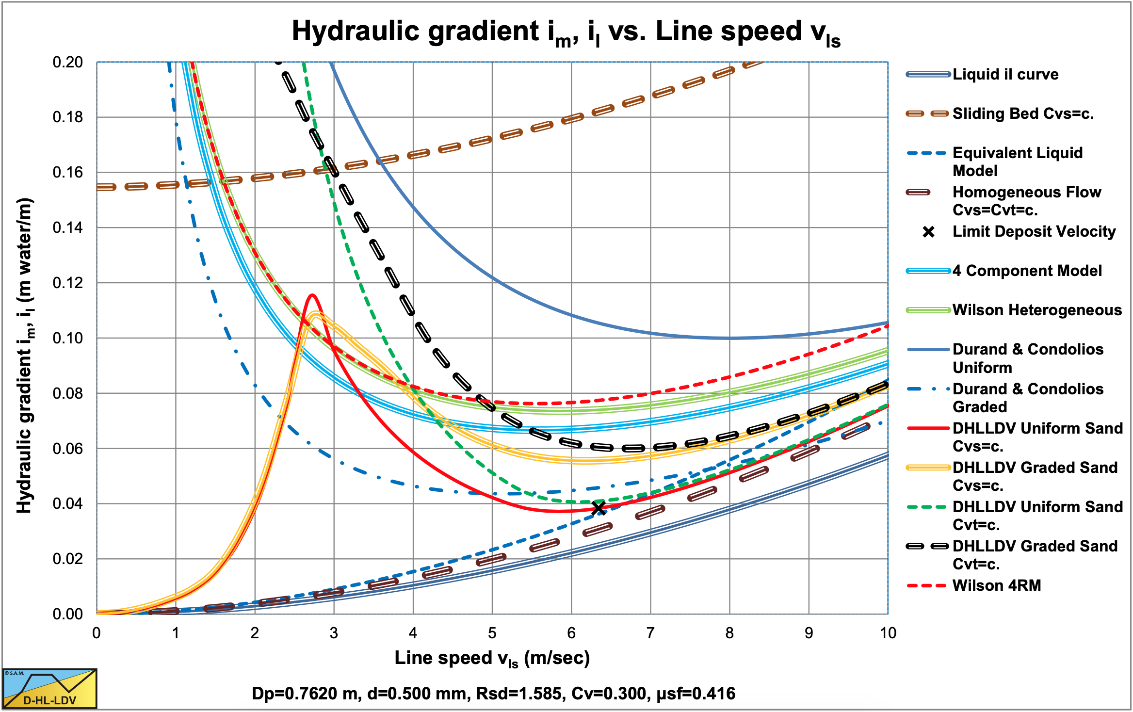
Figure 9.5-10 shows the PSD’s of the original sand, the PSD of the heterogeneous fraction of the 4CM, the corrected PSD of the DHLLDV Framework (without the fines) and the delivered PSD. The delivered PSD has a slightly smaller d₅₀, due to the slip velocity of the particles. Very small particles have a smaller slip velocity than larger particles.

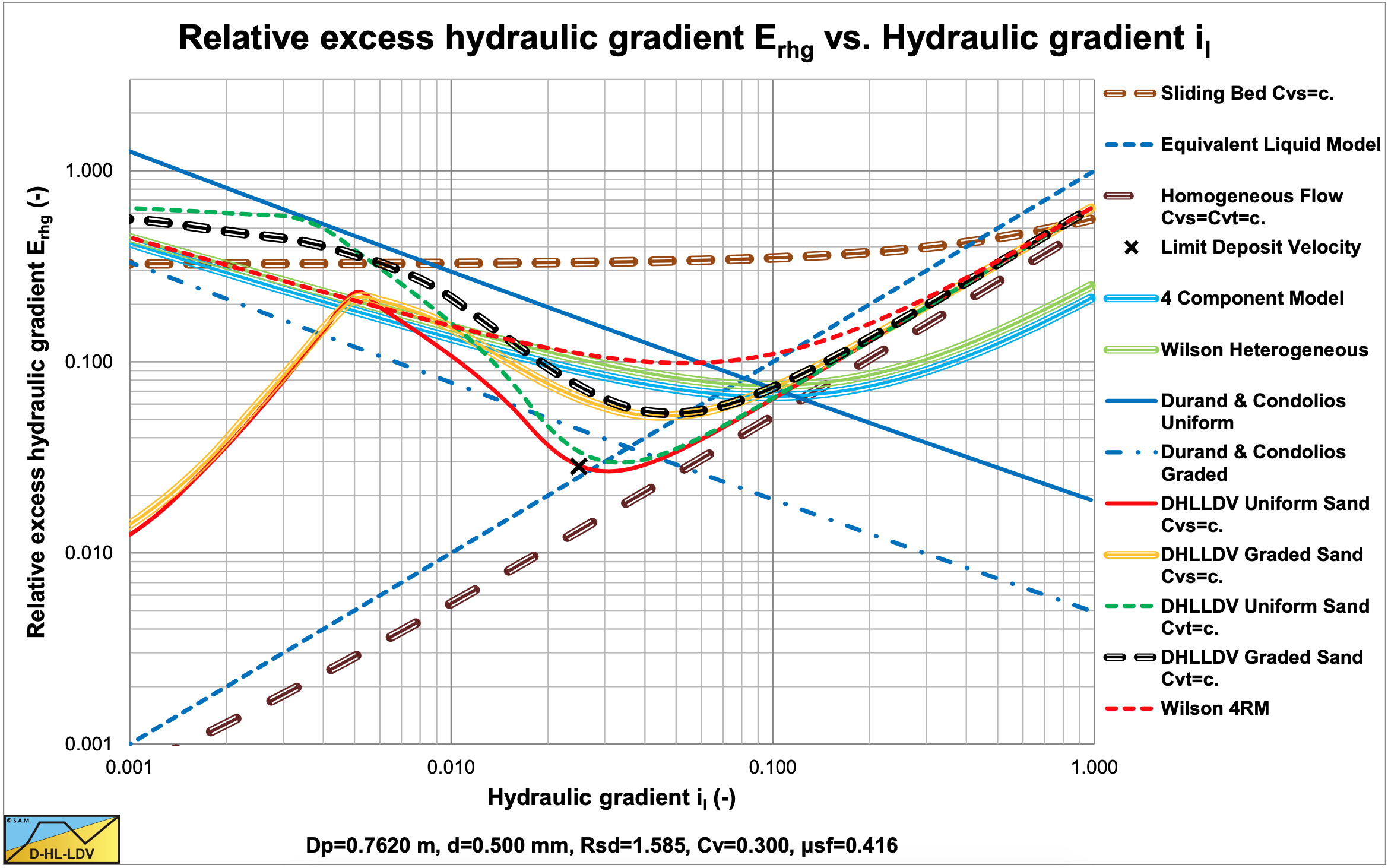
Figure 9.5-11 and Figure 9.5-12 show the hydraulic gradient curves and the solids effect curves. In this larger pipe the Wilson and 4CM curves are higher than the DHLLDV Framework curve. The main reason is the implementation of near wall lift in the DHLLDV Framework and the absence of the sliding flow regime, resulting in a sharper decrease of the hydraulic gradient and solids effect near the transition heterogeneous flow regime and homogeneous flow regime. The Wilson models and 4CM do not incorporate these effects, resulting in an almost pipe diameter independent shape of the curves.

Figure 9.5-12: The resulting relative excess hydraulic gradient curves, also named the stratification ratio, D_p=0.762 m.

9.5.6 Conclusions & Discussion

The Durand & Condolios (1952) model always gives a lower hydraulic gradient curve for graded sands or gravels, compared with uniform sand or gravel, which contradicts with the 3 other methods. This is caused by the shape of the √C_x number graph in Figure 6.4-20. In the example considered the value increases from 1.13 for uniform sand (the thin solid blue line) to 3.54 for graded sand (the thin dash dot blue line). The effect of this is a reduction to 20% of the solids effect in the hydraulic gradient for the graded sand. This does not seem to be reasonable and also contradicts measurements of Clift et al. (1982) with broad graded crushed granite, which matches the other 3 methods.

For the D_p=0.1524 m pipe diameter, the Limit Deposit Velocity, the line speed above which there is no stationary or sliding bed, is estimated by the DHLLDV Framework to be about 3.1 m/s. Under operational conditions, line speeds in the range of 3-5 m/s in the pipe diameter considered, the Wilson heterogeneous model (thick green solid line), the 4CM model (thick light blue solid line) and the DHLLDV Framework (thick dashed black line) give very similar hydraulic gradients and E_rhg curves, of which the 4CM gives a slightly higher hydraulic gradient.

The DHLLDV Framework has 10.3% of the particles to adjust the carrier liquid properties, which is a 3% concentration in the case considered (30% solids). About 16.3% of the particles are in the sliding flow regime, which is an integral part of the Framework. The original Wilson heterogeneous model gives a power M=0.587, the simplified model M=0.621. For the 4CM model a power of M=1 is applied, according to Sellgren et al. (2016). The 4CM has about 6% of the particles in the homogeneous component (1.8% concentration), 21% in the pseudo homogeneous component, 57% in the heterogeneous component and 16% in the fully stratified component. For both the DHLLDV Framework and the 4CM, the carrier liquid properties were adjusted, but only slightly.

The differences between the 3 models occur outside the operational line speed range. The solids effect of the Wilson heterogeneous model and the 4 CM go to infinity for very small line speeds, due to the formulation of the heterogeneous component, see equation (9.5-21) and equation (9.5-33) for the stratified component in the 4CM.

The solids effect of the Wilson heterogeneous model goes to zero at very high line speeds, see also equation (9.5-21). The solids effect of the 4CM will increase at very high line speeds due to the effects of the homogeneous and pseudo homogeneous fractions. The 4CM curve would be a bit lower if the reduced relative submerged density was used as in the original model.

The D_p=0.762 m pipe simulations show a difference between the models. Here the LDV is about 6.3 m/s and the operational range from 6 m/s to 9 m/s. The DHLLDV Framework curve is much lower than Wilson 4RM (highest), the Wilson heterogeneousand the Wilson & Sellgren 4CM.

The Durand & Condolios model contradicts with these 4 models and is rejected.

The main difference between the 4CM and the DHLLDV Framework is, the 4CM uses fixed boundaries based on particle diameters to divide the PSD into 4 components. These boundaries do not depend on the line speed. The DHLLDV Framework determines the hydraulic gradient curves for each fraction separately. The result is a changing flow regime division depending on the line speed and the particle diameter. Particles that may be in a sliding bed at low line speeds, behave heterogeneous at a higher line speed and homogeneous at a very high line speed. Here the PSD is divided into 9 fractions, which seems to be enough, however the number of fractions can be unlimited.

The concept of the v₅₀ pivot point of Wilson, the heterogeneous line of Wilson in the E_rhg graph pivots around the v₅₀ when the power M is changed, matched the results of the DHLLDV Framework. At line speeds higher than the v₅₀ the solids effect increases while at lower line speeds it decreases with increased grading, although the line speed of this pivot point is not exactly the same in both models, but it is close.

Under operational conditions all 4 models, the Wilson heterogeneous model, the Wilson 4RM, the Sellgren & Wilson 4CM and the DHLLDV Framework, can be used for small pipe diameters. Outside the operational conditions, low and high line speeds, the DHLLDV Framework takes the behavior of a possible sliding bed and homogeneous flow better into account. For large pipe diameters the 4 models differ. However there are no experimental data proving which model is the best.

Only the Wilson 4RM and the DHLLDV Framework match all criteria from the beginning of this chapter.

As final remarks it should be stated that the interaction between fractions and/or components is not taken into account and could influence the outcome. The use of the delivered volumetric concentration for a graded sand or gravel is not very convenient since the delivered PSD does not have to be the same as the spatial PSD.

9.5.7 Nomenclature Graded Sands & Gravels

Ax, A15, A85	Factor PSD	-
A	Correction factor pseudo homogeneous flow	-
B	Correction factor stratified flow	-
Cvs	Spatial volumetric concentration	-
Cvt	Delivered/transport volumetric concentration	-
Cvb	Volumetric bed concentration	-
Cvs,r	Remaining spatial volumetric concentration	-
Cvs,x	Volumetric concentration of fraction x	-
Cx	Durand & Condolios particle drag coefficient	-
CD	Particle drag coefficient	-
d	Particle diameter	m
dx, dy	Particle diameter	m
d50	Particle diameter 50% passing by weight	m
d15, d85	Particle diameter 15%/85% passing by weight	m
dlim	Limiting particle diameter homogeneous fraction	m
Dp	Pipe diameter	m
Erhg	Relative excess hydraulic gradient (stratification ratio)	-
f	Correction factor determination v50	-
fy, fx	Fraction passing	-
Fr	Froude number	-
g	Gravitational constant	m/s^2
il	Hydraulic gradient liquid	-
im	Hydraulic gradient mixture	-
if	Hydraulic gradient adjusted carrier liquid	-
K	Durand & Condolios constant	-
ΔL	Length of pipeline	m
M	Power Wilson heterogeneous equation (0.25-1.7)	-
n	Porosity	-
NWL	Near Wall Lift	-
dp, pi	Probability	-
Δpl	Liquid pressure	kPa
Δpm	Mixture pressure	kPa
R	Stratification ratio (Erhg)	-
Rsd	Relative submerged density	-
Rsd,f	Relative submerged density in adjusted carrier liquid	-
Sf	Relative density adjusted carrier liquid	-
Stk	Stokes number	-
vls	Line speed	m/s
vls,ldv	Limit Deposit Velocity	m/s
v50	50% stratification ratio line speed for d50	m/s
v50,f	50% stratification ratio line speed for d50 in adjusted carrier liquid	m/s
vt	Terminal settling velocity particle	m/s
vsm	Maximum Limit of Stationary Deposit Velocity	m/s
vsm,f	Maximum Limit of Stationary Deposit Velocity in adjusted carrier liquid	m/s
w50	Particle associated velocity Wilson for d50	m/s
w85	Particle associated velocity Wilson for d85	m/s
X	Fraction	-
Xf	Fraction of PSD in homogeneous component	-
Xph	Fraction of PSD in pseudo homogeneous component	-
Xh	Fraction of PSD in heterogeneous component	-
Xs	Fraction of PSD in fully stratified component	-
α15, α85	Ratio	-
β	Bed angle with vertical	rad
λl	Darcy Weisbach friction coefficient liquid	-
λf	Darcy Weisbach friction coefficient adjusted carrier liquid	-
ρl	Liquid density	ton/m^3
ρs	Solids density	ton/m^3
ρx	Pseudo liquid density	ton/m^3
ρm	Mixture density	ton/m^3
σ	Variance PSD	-
\(\ v_{\mathrm{l}}, v_{\mathrm{w}} \)	Kinematic viscosity liquid/water	m^2/s
\(\ v_{\mathrm{x}} \)	Kinematic viscosity pseudo liquid	m^2/s
μl	Dynamic viscosity liquid	Pa·s
μx	Dynamic viscosity pseudo liquid	Pa·s
μsf	Sliding friction factor	-
Φ	Durand & Condolios solids effect	-
ψ	Durand & Condolios solids effect	-
ξ	Slip ratio	-
ξvsm	Slip ratio at vsm	-