2.5: Criteria and Concepts

2.5.1. Failure Criteria

After a soil reaches the critical state, it is no longer contracting or dilating and the shear stress on the failure plane τ_crit is determined by the effective normal stress on the failure plane σ_n' and critical state friction angle, φ_cv, :

\[\ \mathrm{ \tau_{\text {crit }}=\sigma_{n}^{\prime} \cdot \tan \left(\varphi_{c v}\right)}\tag{2-31}\]

The peak strength of the soil may be greater, however, due to the interlocking (dilatancy) contribution. This may be stated:

\[\ \tau_{\text {peak }}=\sigma_{\mathrm{n}}^{\prime} \cdot \tan \left(\varphi_{\text {peak }}\right)\tag{2-32}\]

Where φ_peak > φ_cv. However, use of a friction angle greater than the critical state value for design requires care. The peak strength will not be mobilized everywhere at the same time in a practical problem such as a foundation, slope or retaining wall. The critical state friction angle is not nearly as variable as the peak friction angle and hence it can be relied upon with confidence. Not recognizing the significance of dilatancy, Coulomb proposed that the shear strength of soil may be expressed as a combination of adhesion and friction components:

\[\ \mathrm{\tau=\sigma^{\prime} \cdot \tan (\varphi)+c^{\prime}}\tag{2-33}\]

It is now known that the c' and φ parameters in the last equation are not fundamental soil properties. In particular, c' and φ are different depending on the magnitude of effective stress. According to Schofield (2006), the longstanding use of c' in practice has led many engineers to wrongly believe that c' is a fundamental parameter. This assumption that c' and φ are constant can lead to overestimation of peak strengths.

2.5.2. The Phi=0 Concept

When a fast triaxial test is carried out, so an unconsolidated undrained test, it is very well possible that the pore pressures will be equal to the increase of the cell pressure. If a test at high cell pressure is carried out, the only difference with a test with a low cell pressure is the value of the pore pressures. The grain pressures will be almost equal in both cases and the result is, that we will find the same critical Mohr circle. So let’s consider a series of unconsolidated undrained (UU) tests. Three specimens are selected and all are consolidated to 110 kPa. This brings the specimens to the end of step 1 in the UU test program. Now the confining pressures are changed to say 70, 140 and 700 kPa, without allowing further consolidation and the sheared undrained. The result, within experimental scatter, is that the shear stress or radius of the Mohr circle is about 35 kPa for each specimen.

So what happened?

When the confining pressure was changed, the pore pressure in the fully saturated specimens changed just as much as did the confining pressure, and the effective stress remained unchanged and equal in each specimen. Thus the effective stress remained 110 kPa and each specimen behaved during shear just as did the CU specimen. The shear stress and thus the radius of the Mohr circle did not increase and apparently the specimens did not encounter internal friction. This is called the phi=0 concept. In clays with a very low permeability and at a high deformation rate, like during the cutting of clay, the clay behaves like the internal friction angle is zero. So for cutting processes the phi=0 concept will be applied.

2.5.3. Factors Controlling Shear Strength of Soils

The stress-strain relationship of soils, and therefore the shearing strength, is affected by:

1. Soil composition (basic soil material): mineralogy, grain size and grain size distribution, shape of particles, pore fluid type and content, ions on grain and in pore fluid.

2. State (initial): Defined by the initial void ratio, effective normal stress and shear stress (stress history). State can be described by terms such as: loose, dense, over consolidated, normally consolidated, stiff, soft, contractive, dilative, etc.

3. Structure: Refers to the arrangement of particles within the soil mass; the manner the particles are packed or distributed. Features such as layers, joints, fissures, slickensides, voids, pockets, cementation, etc., are part of the structure. Structure of soils is described by terms such as: undisturbed, disturbed, remolded, compacted, cemented; flocculent, honey-combed, single-grained; flocculated, deflocculated; stratified, layered, laminated; isotropic and anisotropic.

4. Loading conditions: Effective stress path, i.e., drained, and undrained; and type of loading, i.e., magnitude, rate (static, dynamic), and time history (monotonic, cyclic).

The shear strength and stiffness of soil determines whether or not soil will be stable or how much it will deform. Knowledge of the strength is necessary to determine if a slope will be stable, if a building or bridge might settle too far into the ground, and the limiting pressures on a retaining wall. It is important to distinguish between failure of a soil element and the failure of a geotechnical structure (e.g., a building foundation, slope or retaining wall); some soil elements may reach their peak strength prior to failure of the structure. Different criteria can be used to define the "shear strength" and the "yield point" for a soil element from a stress-strain curve. One may define the peak shear strength as the peak of a stress strain curve, or the shear strength at critical state as the value after large strains when the shear resistance levels off. If the stress-strain curve does not stabilize before the end of shear strength test, the "strength" is sometimes considered to be the shear resistance at 15% to 20% strain. The shear strength of soil depends on many factors including the effective stress and the void ratio.

The shear stiffness is important, for example, for evaluation of the magnitude of deformations of foundations and slopes prior to failure and because it is related to the shear wave velocity. The slope of the initial, nearly linear, portion of a plot of shear stress as a function of shear strain is called the shear modulus

2.5.4. Friction, Interlocking & Dilation

Soil is an assemblage of particles that have little to no cementation while rock (such as sandstone) may consist of an assembly of particles that are strongly cemented together by chemical bonds. The shear strength of soil is primarily due to inter-particle friction and therefore, the shear resistance on a plane is approximately proportional to the effective normal stress on that plane. [3] But soil also derives significant shear resistance from interlocking of strain. The expansion of the particle matrix due to shearing was called dilatancy by Osborne Reynolds. If one considers the energy required to shear an assembly of particles there is energy input by the shear force, T, moving a distance, x and there is also energy input by the normal force, N, as the sample expands a distance, y. Due to the extra energy required for the particles to dilate against the confining pressures, dilatant soils have greater peak strength than contractive soils. Furthermore, as dilative soil grains dilate, they become looser (their void ratio increases), and their rate of dilation decreases until they reach a critical void ratio. Contractive soils become denser as they shear, and their rate of contraction decreases until they reach a critical void ratio.

The tendency for a soil to dilate or contract depends primarily on the confining pressure and the void ratio of the soil. The rate of dilation is high if the confining pressure is small and the void ratio is small. The rate of contraction is high if the confining pressure is large and the void ratio is large. As a first approximation, the regions of contraction and dilation are separated by the critical state line.

2.5.5. Effective Stress

Karl von Terzaghi (1964) first proposed the relationship for effective stress in 1936. For him, the term ‘effective’ meant the calculated stress that was effective in moving soil, or causing displacements. It represents the average stress carried by the soil skeleton. Effective stress (σ') acting on a soil is calculated from two parameters, total stress (σ) and pore water pressure (u) according to:

\[\ \sigma^{\prime}=\sigma-\mathrm{u}\tag{2-34}\]

Typically, for simple examples:

\[\ \sigma=\gamma_{\mathrm{soil}} \cdot \mathrm{H}_{\mathrm{soil}}\quad\text{ and }\quad\mathrm{u}=\gamma_{\mathrm{w}} \cdot \mathrm{H}_{\mathrm{w}}\tag{2-35}\]

Much like the concept of stress itself, the formula is a construct, for the easier visualization of forces acting on a soil mass, especially simple analysis models for slope stability, involving a slip plane. With these models, it is important to know the total weight of the soil above (including water), and the pore water pressure within the slip plane, assuming it is acting as a confined layer.

However, the formula becomes confusing when considering the true behavior of the soil particles under different measurable conditions, since none of the parameters are actually independent actors on the particles.

Consider a grouping of round quartz sand grains, piled loosely, in a classic ‘cannonball’ arrangement. As can be seen, there is a contact stress where the spheres actually touch. Pile on more spheres and the contact stresses increase, to the point of causing frictional instability (dynamic friction), and perhaps failure. The independent parameter affecting the contacts (both normal and shear) is the force of the spheres above. This can be calculated by using the overall average density of the spheres and the height of spheres above.

If we then have these spheres in a beaker and add some water, they will begin to float a little depending on their density (buoyancy). With natural soil materials, the effect can be significant, as anyone who has lifted a large rock out of a lake can attest. The contact stress on the spheres decreases as the beaker is filled to the top of the spheres, but then nothing changes if more water is added. Although the water pressure between the spheres (pore water pressure) is increasing, the effective stress remains the same, because the concept of 'total stress' includes the weight of all the water above. This is where the equation can become confusing, and the effective stress can be calculated using the buoyant density of the spheres (soil), and the height of the soil above.

The concept of effective stress truly becomes interesting when dealing with non-hydrostatic pore water pressure. Under the conditions of a pore pressure gradient, the ground water flows, according to the permeability equation (Darcy's law). Using our spheres as a model, this is the same as injecting (or withdrawing) water between the spheres. If water is being injected, the seepage force acts to separate the spheres and reduces the effective stress. Thus, the soil mass becomes weaker. If water is being withdrawn, the spheres are forced together and the effective stress increases. Two extremes of this effect are quicksand, where the groundwater gradient and seepage force act against gravity; and the 'sandcastle effect', where the water drainage and capillary action act to strengthen the sand. As well, effective stress plays an important role in slope stability, and other geotechnical engineering and engineering geology problems, such as groundwater-related subsidence.

2.5.6. Pore Water Pressure: Hydrostatic Conditions

If there is no pore water flow occurring in the soil, the pore water pressures will be hydrostatic. The water table is located at the depth where the water pressure is equal to the atmospheric pressure. For hydrostatic conditions, the water pressure increases linearly with depth below the water table:

\[\ \mathrm{u}=\rho_{\mathrm{w}} \cdot \mathrm{g} \cdot \mathrm{z}_{\mathrm{w}}\tag{2-36}\]

2.5.7. Pore Water Pressure: Capillary Action

Due to surface tension water will rise up in a small capillary tube above a free surface of water. Likewise, water will rise up above the water table into the small pore spaces around the soil particles. In fact the soil may be completely saturated for some distance above the water table. Above the height of capillary saturation, the soil may be wet but the water content will decrease with elevation. If the water in the capillary zone is not moving, the water pressure obeys the equation of hydrostatic equilibrium, u = ρ_w·g·z_w, but note that z_w, is negative above the water table. Hence, hydrostatic water pressures are negative above the water table. The thickness of the zone of capillary saturation depends on the pore size, but typically, the heights vary between a centimeter or so for coarse sand to tens of meters for a silt or clay.

The surface tension of water explains why the water does not drain out of a wet sand castle or a moist ball of clay. Negative water pressures make the water stick to the particles and pull the particles to each other, friction at the particle contacts make a sand castle stable. But as soon as a wet sand castle is submerged below a free water surface, the negative pressures are lost and the castle collapses. Considering the effective stress equation, σ' = σ − u,, if the water pressure is negative, the effective stress may be positive, even on a free surface (a surface where the total normal stress is zero). The negative pore pressure pulls the particles together and causes compressive particle to particle contact forces.

Negative pore pressures in clayey soil can be much more powerful than those in sand. Negative pore pressures explain why clay soils shrink when they dry and swell as they are wetted. The swelling and shrinkage can cause major distress, especially to light structures and roads.

2.5.8. Darcy’s Law

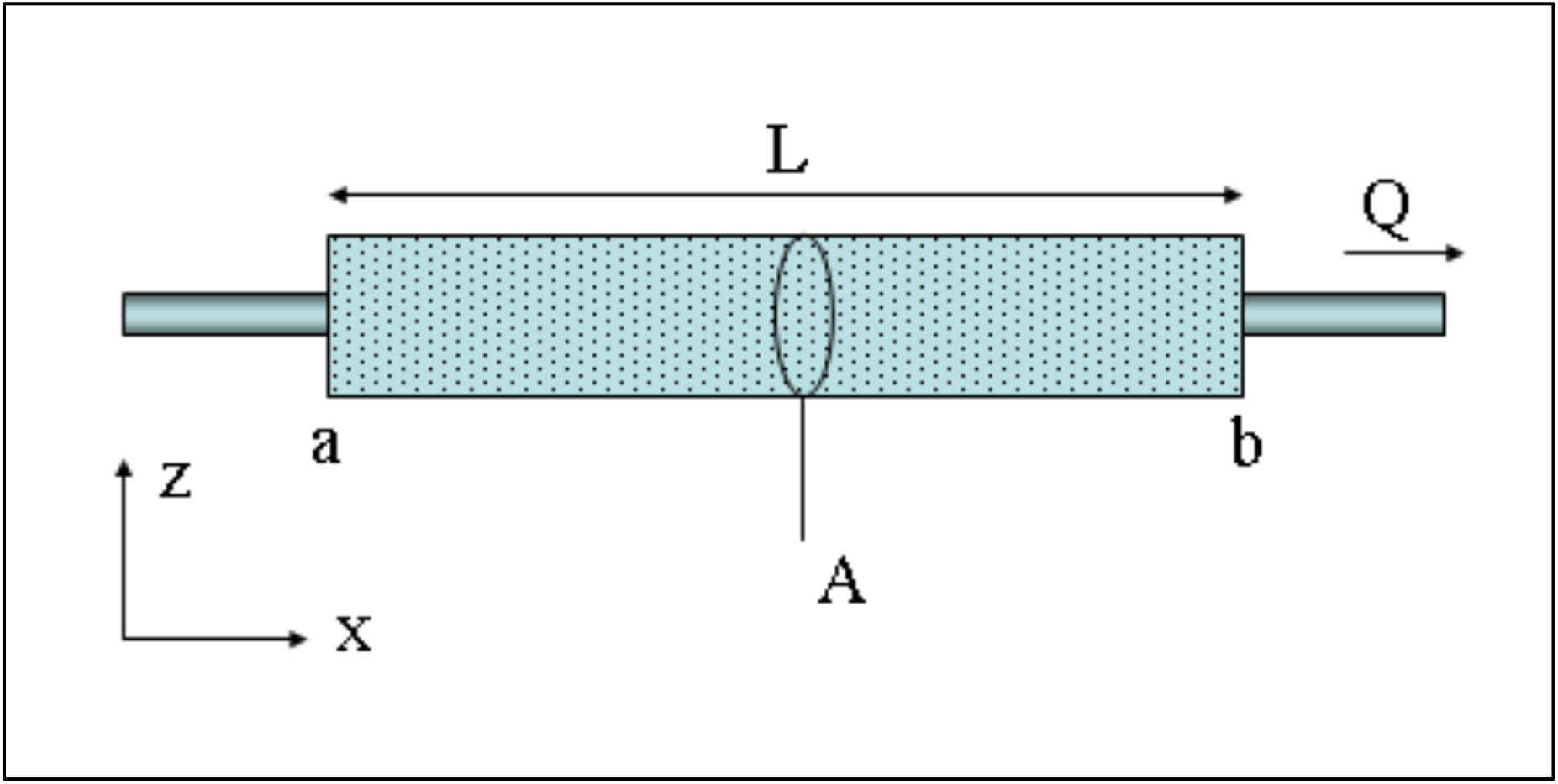
Darcy's law states that the volume of flow of the pore fluid through a porous medium per unit time is proportional to the rate of change of excess fluid pressure with distance. The constant of proportionality includes the viscosity of the fluid and the intrinsic permeability of the soil.

\[\ \mathrm{Q}=\frac{-\mathrm{K} \cdot \mathrm{A}}{\mu_{\mathrm{l}}} \cdot \frac{\left(\mathrm{u}_{\mathrm{b}}-\mathrm{u}_{\mathrm{a}}\right)}{\mathrm{L}}\tag{2-37}\]

The negative sign is needed because fluids flow from high pressure to low pressure. So if the change in pressure is negative (in the x-direction) then the flow will be positive (in the x-direction). The above equation works well for a horizontal tube, but if the tube was inclined so that point b was a different elevation than point a, the equation would not work. The effect of elevation is accounted for by replacing the pore pressure by excess pore pressure, u_e defined as:

\[\ \mathrm{u}_{\mathrm{c}}=\mathrm{u}-\rho_{\mathrm{w}} \cdot \mathrm{g} \cdot \mathrm{z}\tag{2-38}\]

Where z is the depth measured from an arbitrary elevation reference (datum). Replacing u by u_e we obtain a more general equation for flow:

\[\ \mathrm{Q}=\frac{-\mathrm{K} \cdot \mathrm{A}}{\mu_{\mathrm{l}}} \cdot \frac{\left(\mathrm{u}_{\mathrm{c}, \mathrm{b}}-\mathrm{u}_{\mathrm{c}, \mathrm{a}}\right)}{\mathrm{L}}\tag{2-39}\]

Figure 2-27: Diagram showing definitions and directions for Darcy’s law.

Dividing both sides of the equation by A, and expressing the rate of change of excess pore pressure as a derivative, we obtain a more general equation for the apparent velocity in the x-direction:

\[\ \mathrm{q_{x}=\frac{-K}{\mu_{l}} \cdot \frac{d u_{c}}{d x}}\tag{2-40}\]

Where qx has units of velocity and is called the Darcy velocity, or discharge velocity. The seepage velocity (v_sx = average velocity of fluid molecules in the pores) is related to the Darcy velocity, and the porosity, n:

\[\ \mathrm{\mathrm{v}_{s, \mathrm{x}}=\frac{\mathrm{q}_{\mathrm{x}}}{\mathrm{n}}}\tag{2-41}\]

Civil engineers predominantly work on problems that involve water and predominantly work on problems on earth (in earth’s gravity). For this class of problems, civil engineers will often write Darcy's law in a much simpler form:

\[\ \mathrm{q}_{\mathrm{x}}=\mathrm{k} \cdot \mathrm{i}_{\mathrm{x}}\tag{2-42}\]

Where k is called permeability, and is defined as:

\[\ \mathrm{\mathrm{k}=\mathrm{K} \cdot \frac{\rho_{l} \cdot \mathrm{g}}{\mu_{l}}}\tag{2-43}\]

And i is called the hydraulic gradient. The hydraulic gradient is the rate of change of total head with distance. Values are for typical fresh groundwater conditions, using standard values of viscosity and specific gravity for water at 20°C and 1 atm.

Table 2-14: Typical values of the permeability k.

Soil	Permeability (m/s)	Degree of permeability
Well sorted gravel	10^0>k>10^-2	Extremely high
Gravel	10^-2>k>10^-3	Very high
Sandy gravel, clean sand, fine sand	10^-3>k>10^-5	High to Medium
Sand, dirty sand, silty sand	10^-5>k>10^-7	Low
Silt, silty clay	10^-7>k>10^-9	Very low
Clay	<10^-9	Vitually impermeable
Highly fractured rocks	10^0>k>10^-3	Very high
Oil reservoir rocks	10^-4>k>10^-6	Medium to Low
Fresh sandstone	10^-7>k>10^-8	Very low
Fresh limestone, dolomite	10^-9>k>10^-10	Vitually impermeable
Fresh granite	<10^-11	Vitually impermeable

Table 2-15: Some permeabilities according to Hazen’s equation.

Material	Permeability (m/s)	d10 (mm)
Uniform coarse sand	0.0036	0.6
Uniform medium sand	0.0009	0.3
Clean, well-graded sand	0.0001	0.1
Uniform fine sand	36·10^-6	0.06
Well-graded fine sand	4·10^-6	0.02
Silty sand	10^-6	0.01
Uniform silt	36·10^-8	0.006
Sandy clay	4·10^-8	0.002
Silty clay	10^-8	0.001
Clay	64·10^-10	0.0008
Colloidal clay	9·10^-11	0.00003

2.5.9. Brittle versus Ductile Failure

The terms ductile failure and brittle failure are often used in literature for the failure of materials with shear strength and tensile strength.

“In materials science, ductility is a solid material's ability to deform under tensile stress; this is often characterized by the material's ability to be stretched into a wire. Malleability, a similar property, is a material's ability to deform under compressive stress; this is often characterized by the material's ability to form a thin sheet by hammering or rolling. Both of these mechanical properties are aspects of plasticity, the extent to which a solid material can be plastically deformed without fracture. Ductility and malleability are not always coextensive – for instance, while gold has high ductility and malleability, lead has low ductility but high malleability. The word ductility is sometimes used to embrace both types of plasticity.

A material is brittle if, when subjected to stress, it breaks without significant deformation (strain). Brittle materials absorb relatively little energy prior to fracture, even those of high strength. Breaking is often accompanied by a snapping sound. Brittle materials include most ceramics and glasses (which do not deform plastically) and some polymers, such as PMMA and polystyrene. Many steels become brittle at low temperatures (see ductile-brittle transition temperature), depending on their composition and processing. When used in materials science, it is generally applied to materials that fail when there is little or no evidence of plastic deformation before failure. One proof is to match the broken halves, which should fit exactly since no plastic deformation has occurred. Generally, the brittle strength of a material can be increased by pressure. This happens as an example in the brittle-ductile transition zone at an approximate depth of 10 kilometers in the Earth's crust, at which rock becomes less likely to fracture, and more likely to deform ductile.” (Source Wikipedia).

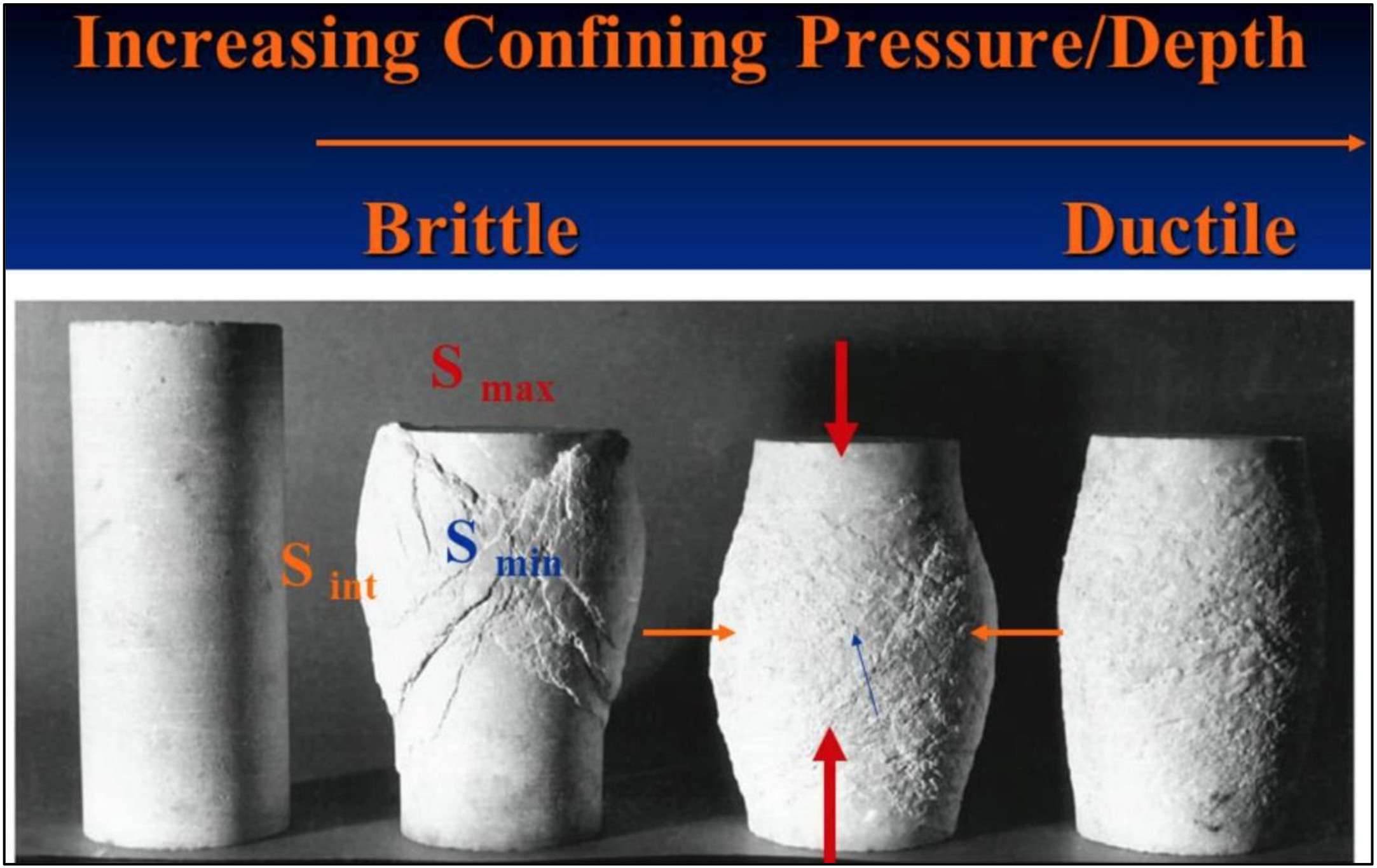
In rock failure a distinction is made between brittle, brittle ductile and ductile failure. Factors determining those types of failure are the ductility number (ratio compressive strength over tensile strength), the confining pressure and the temperature. During dredging the temperature will have hardly any influence, however when drilling deep oil wells temperature will play an important role. The confining pressure, where the failure transit from brittle to ductile is called σ_bp.

Figure 2-28: Brittle failure types (Vlasblom (2003-2007)).

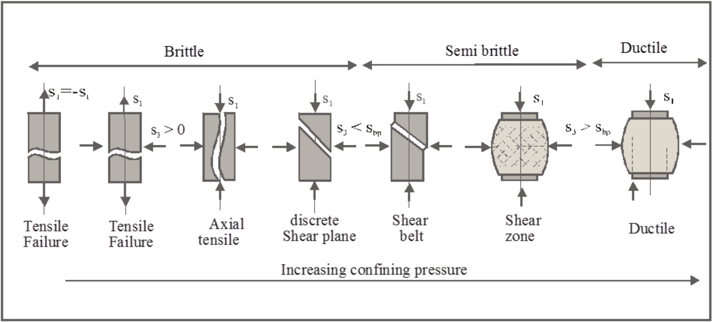
Brittle failure occurs at relative low confining pressures σ₃ < σ_bp en deviator stress q=σ₁-σ₃ > 1⁄2q_u. The strength increases with the confining pressure, but decreases after the peak strength to a residual value. The presence of pore water can play an important role.

Brittle failure types are:

• Pure tensile failure with or without a small confining pressure.

• Axial tensile failure

• Shear plane failure

Brittle ductile failure is also called semi brittle. In the transition area where σ₃ \(\ \approx \) σ_bp, the deformations are not restricted to local shear planes or fractures but are divided over the whole area. The residual- strength is more or less equal to the peak strength.

Ductile failure. A rock fails ductile when σ₃ >> q_u and σ₃ > σ_bp while the force stays constant or increases some what with increasing deformation.

Figure 2-29: Brittle-ductile failure of marble (M.S. Patterson, Australian National University).