2.8: The Mohr Circle

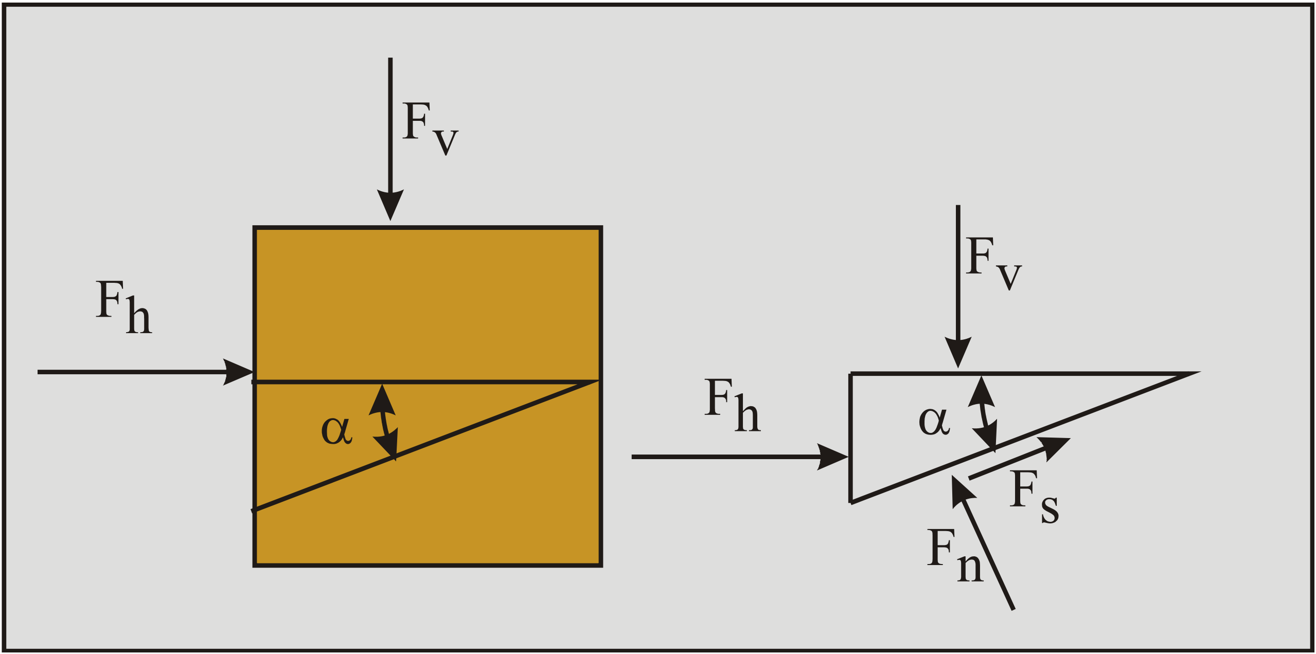
In the derivation of the Mohr circle the vertical stress σ_v and the horizontal stress σ_h are assumed to be the principal stresses, but in reality these stresses could have any orientation. It should be noted here that the Mohr circle approach is valid for the stress situation in a point in the soil. Now consider an infinitesimal element of soil under plane strain conditions as is shown in Figure 2-44. On the element a vertical stress σ_v and a horizontal stress σ_h are acting. On the horizontal and vertical planes the shear stresses are assumed to be zero. Now the question is, what would the normal stress σ and shear stress \(\ \tau\) be on a plane with an angle α with the horizontal direction? To solve this problem, the horizontal and vertical equilibriums of forces will be derived. Equilibriums of stresses do not exist. One should consider that the surfaces of the triangle drawn in Figure 2-44 are not equal. If the surface (or length) of the surface under the angle α is considered to be 1, then the surface (or length) of the horizontal side is cos(α) and the vertical side sin(α). The stresses have to be multiplied with their surface in order to get forces and forces are required for the equilibriums of forces, see Figure 2-45. The derivation of the Mohr circle is also an exercise for the derivation of many equations in this book where equilibriums of forces and moments are applied.

Figure 2-44: The stresses on a soil element.

Figure 2-45: The forces on a soil element.

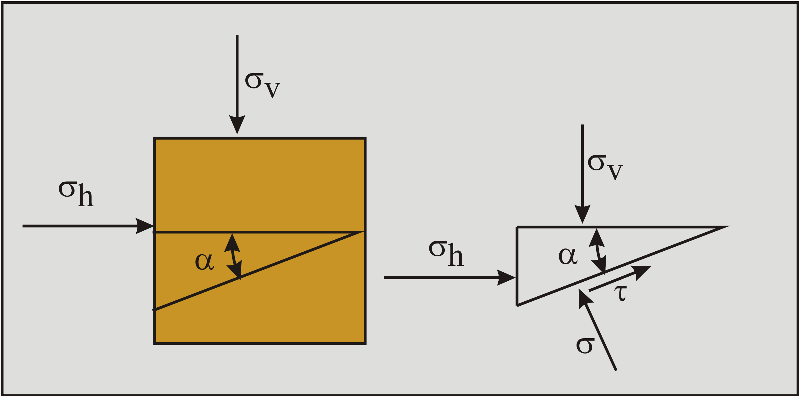
Since an equilibrium of stresses does not exist, only an equilibrium of forces exists, the forces on the soil element have to be known, or the ratio of the forces has to be known.

These forces are, assuming the length of the side under an angle α is 1:

\[\ \mathrm{F}_{\mathrm{h}}=\sigma_{\mathrm{h}} \cdot \sin (\alpha)\quad\text{ and }\quad\mathrm{F}_{\mathrm{v}}=\sigma_{\mathrm{v}} \cdot \cos (\alpha)\tag{2-45}\]

And:

\[\ \mathrm{F}_{\mathrm{n}}=\sigma \quad\text{ and }\quad \mathrm{F}_{\mathrm{s}}=\tau\tag{2-46}\]

The equilibrium of forces in the horizontal direction:

\[\ \begin{array}{left}\mathrm{F_{h}=F_{n} \cdot \sin (\alpha)-F_{s} \cdot \cos (\alpha)}\\
\mathrm{\sigma_{h} \cdot \sin (\alpha)=\sigma \cdot \sin (\alpha)-\tau \cdot \cos (\alpha)}\end{array}\tag{2-47}\]

The equilibrium of forces in the vertical direction:

\[\ \begin{array}{left}\mathrm{F_{v}=F_{n} \cdot \cos (\alpha)+F_{s} \cdot \sin (\alpha)}\\
\mathrm{\sigma_{v} \cdot \cos (\alpha)=\sigma \cdot \cos (\alpha)+\tau \cdot \sin (\alpha)}\end{array}\tag{2-48}\]

Equations (2-47) and (2-48) form a system of two equations with two unknowns σ and \(\ \tau\). The normal stresses σ_h and σ_v are considered to be known variables. To find a solution for the normal stress σ on the plane considered, equation (2-47) is multiplied with sin(α) and equation (2-48) is multiplied with cos(α), this gives:

\[\ \mathrm{\sigma_{h} \cdot \sin (\alpha) \cdot \sin (\alpha)=\sigma \cdot \sin (\alpha) \cdot \sin (\alpha)-\tau \cdot \cos (\alpha) \cdot \sin (\alpha)}\tag{2-49}\]

\[\ \mathrm{\sigma_{v} \cdot \cos (\alpha) \cdot \cos (\alpha)=\sigma \cdot \cos (\alpha) \cdot \cos (\alpha)+\tau \cdot \sin (\alpha) \cdot \cos (\alpha)}\tag{2-50}\]

Adding up equations (2-49) and (2-50) eliminates the terms with τ and preserves the terms with σ, giving:

\[\ \mathrm{\sigma_{v} \cdot \cos ^{2}(\alpha)+\sigma_{h} \cdot \sin ^{2}(\alpha)=\sigma}\tag{2-51}\]

Using some basic rules from trigonometry:

\[\ \cos ^{2}(\alpha)=\frac{1+\cos (2 \cdot \alpha)}{2}\tag{2-52}\]

\[\ \sin ^{2}(\alpha)=\frac{1-\cos (2 \cdot \alpha)}{2}\tag{2-53}\]

Giving for the normal stress σ on the plane considered:

\[\ \sigma=\left(\frac{\sigma_{\mathrm{v}}+\sigma_{\mathrm{h}}}{2}\right)+\left(\frac{\sigma_{\mathrm{v}}-\sigma_{\mathrm{h}}}{2}\right) \cdot \cos (2 \cdot \alpha)\tag{2-54}\]

To find a solution for the shear stress τ on the plane considered, equation (2-47) is multiplied with -cos(α) and equation (2-48) is multiplied with sin(α), this gives:

\[\ \mathrm{-\sigma_{h} \cdot \sin (\alpha) \cdot \cos (\alpha)=-\sigma \cdot \sin (\alpha) \cdot \cos (\alpha)+\tau \cdot \cos (\alpha) \cdot \cos (\alpha)}\tag{2-55}\]

\[\ \mathrm{\sigma_{v} \cdot \cos (\alpha) \cdot \sin (\alpha)=\sigma \cdot \cos (\alpha) \cdot \sin (\alpha)+\tau \cdot \sin (\alpha) \cdot \sin (\alpha)}\tag{2-56}\]

Adding up equations (2-55) and (2-56) eliminates the terms with σ and preserves the terms with \( \tau\), giving:

\[\ \mathrm{\left(\sigma_{v}-\sigma_{h}\right) \cdot \sin (\alpha) \cdot \cos (\alpha)=\tau}\tag{2-57}\]

Using the basic rules from trigonometry, equations (2-52) and (2-53), gives for \( \tau\) on the plane considered:

\[\ \tau=\left(\frac{\sigma_{\mathrm{v}}-\sigma_{\mathrm{h}}}{2}\right) \cdot \sin (2 \cdot \alpha)\tag{2-58}\]

Squaring equations (2-54) and (2-58) gives:

\[\ \left(\sigma-\left(\frac{\sigma_{\mathrm{v}}+\sigma_{\mathrm{h}}}{2}\right)\right)^{2}=\left(\frac{\sigma_{\mathrm{v}}-\sigma_{\mathrm{h}}}{2}\right)^{2} \cdot \cos ^{2}(2 \cdot \alpha)\tag{2-59}\]

And:

\[\ \tau^{2}=\left(\frac{\sigma_{\mathrm{v}}-\sigma_{\mathrm{h}}}{2}\right)^{2} \cdot \sin ^{2}(2 \cdot \alpha)\tag{2-60}\]

Adding up equations (2-59) and (2-60) gives:

\[\ \left(\sigma-\left(\frac{\sigma_{\mathrm{v}}+\sigma_{\mathrm{h}}}{2}\right)\right)^{2}+\tau^{2}=\left(\frac{\sigma_{\mathrm{v}}-\sigma_{\mathrm{h}}}{2}\right)^{2} \cdot\left(\sin ^{2}(2 \cdot \alpha)+\cos ^{2}(2 \cdot \alpha)\right)\tag{2-61}\]

This can be simplified to the following circle equation:

\[\ \left(\sigma-\left(\frac{\sigma_{\mathrm{v}}+\sigma_{\mathrm{h}}}{2}\right)\right)^{2}+\tau^{2}=\left(\frac{\sigma_{\mathrm{v}}-\sigma_{\mathrm{h}}}{2}\right)^{2}\tag{2-62}\]

If equation (2-62) is compared with the general circle equation from mathematics, equation (2-63):

\[\ \mathrm{\left(x-x_{C}\right)^{2}+\left(y-y_{C}\right)^{2}=R^{2}}\tag{2-63}\]

The following is found:

\[\ \begin{array}{left}\mathrm{x}=\sigma\\
\mathrm{x}_{\mathrm{C}}=\left(\frac{\sigma_{\mathrm{v}}+\sigma_{\mathrm{h}}}{2}\right)\\
\mathrm{y}=\tau\\
\mathrm{y}_{\mathrm{C}}=\mathrm{0}\\
\mathrm{R}=\left(\frac{\sigma_{\mathrm{v}}-\sigma_{\mathrm{h}}}{2}\right)\end{array}\tag{2-64}\]

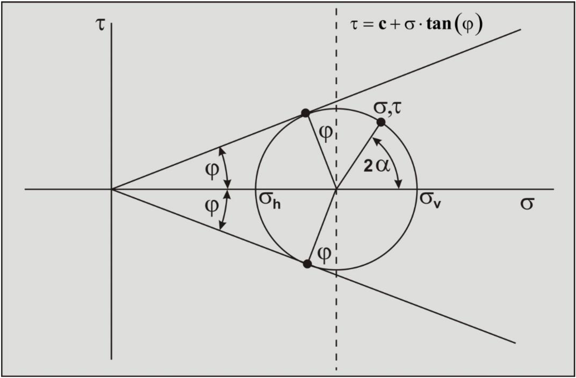
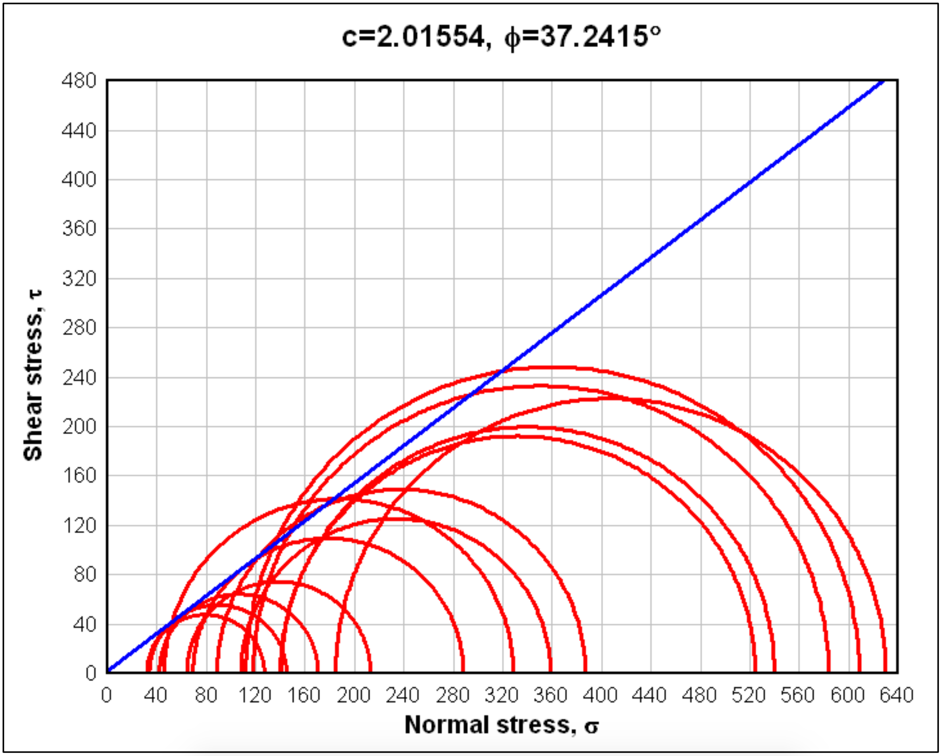
Figure 2-46 shows the resulting Mohr circle with the Mohr-Coulomb failure criterion:

\[\ \tau=\mathrm{c}+\sigma \cdot \tan (\varphi)\tag{2-65}\]

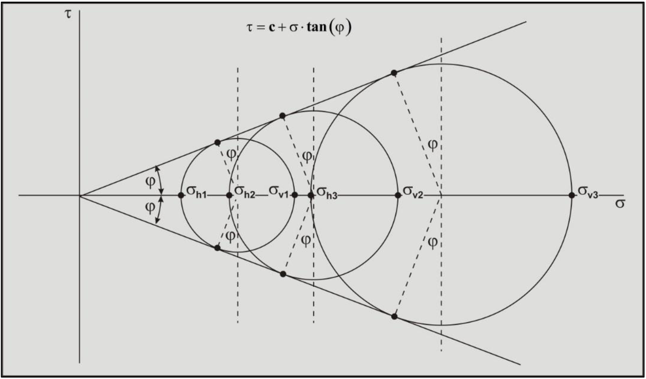
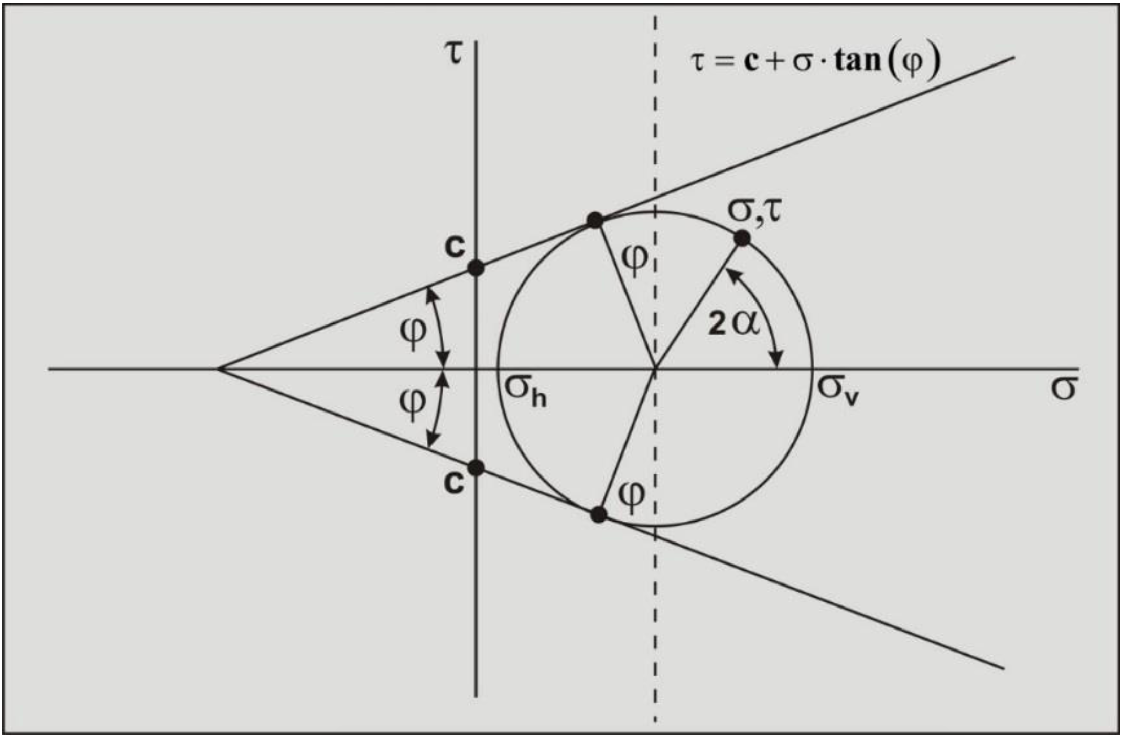
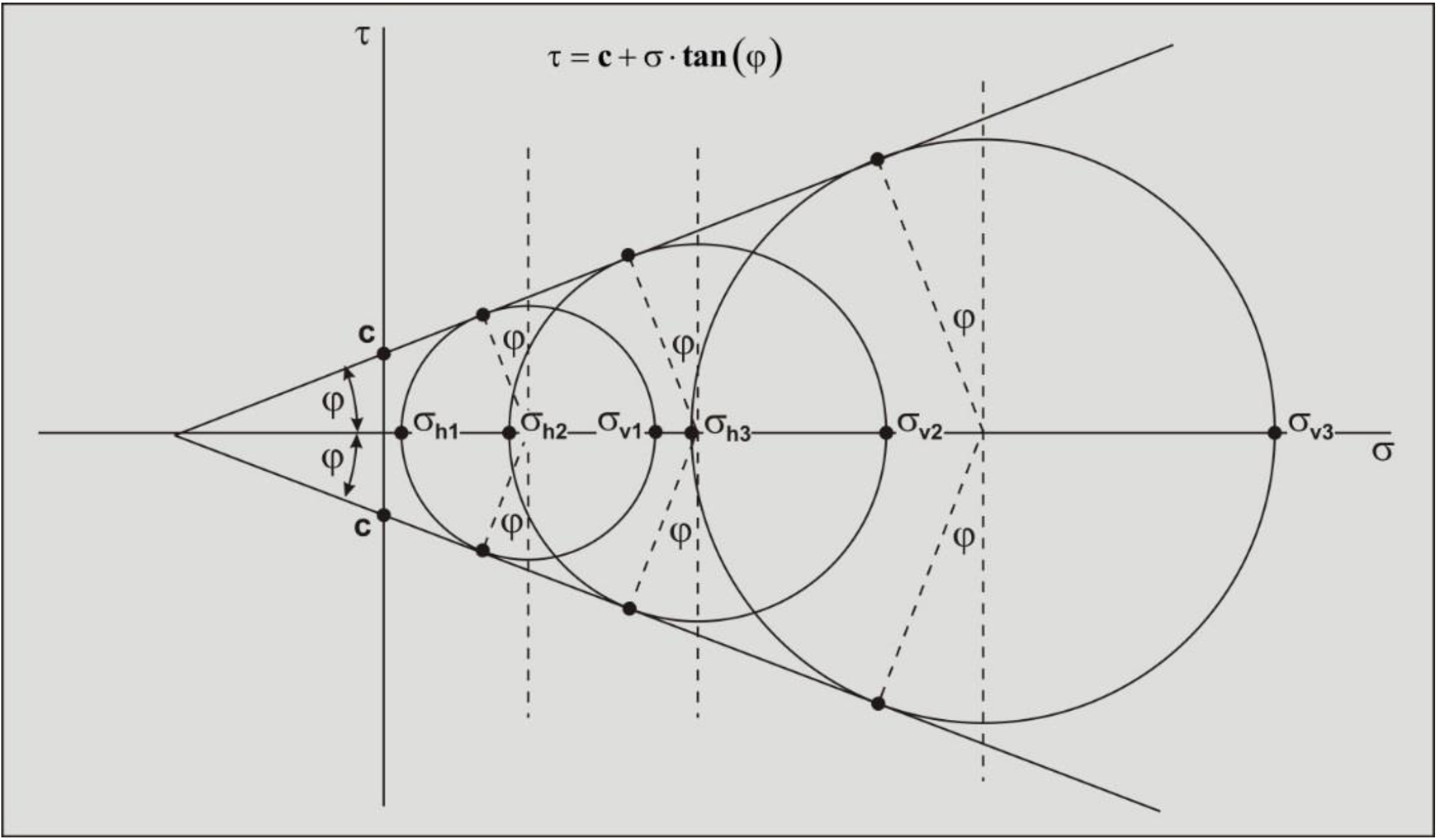
The variable c is the cohesion or internal shear strength of the soil. In Figure 2-46 it is assumed that the cohesion c=0, which describes the behavior of a cohesion less soil, sand. Further it is assumed that the vertical stress σ_v (based on the weight of the soil above the point considered) is bigger than the horizontal stress σ_h. So in this case the horizontal stress at failure follows the vertical stress. The angle α of the plane considered, appears as an angle of 2·α in the Mohr circle. Figure 2-47: shows how the internal friction angle can be determined from a number of tri-axial tests for a cohesion less soil (sand). The 3 circles in this figure will normally not have the failure line as a tangent exactly, but one circle will be a bit too big and another a bit too small. The failure line found will be a best fit. Figure 2-48 and Figure 2-49 show the Mohr circles for a soil with an internal friction angle and cohesion. In such a soil, the intersection point of the failure line with the vertical axis is considered to be the cohesion.

Figure 2-46: The resulting Mohr circle for cohesion less soil.

Figure 2-47: Determining the angle of internal friction from tri-axial tests of cohesion less soil.

Figure 2-48: The Mohr circle for soil with cohesion.

Figure 2-49: Determining the angle of internal friction from tri-axial tests of soil with cohesion.

Figure 2-50: An example of Mohr circles resulting in an internal friction angle and cohesion (www.dplot.com).