7.8: Experiments in Clay

7.8.1. Experiments of Hatamura & Chijiiwa (1977B)

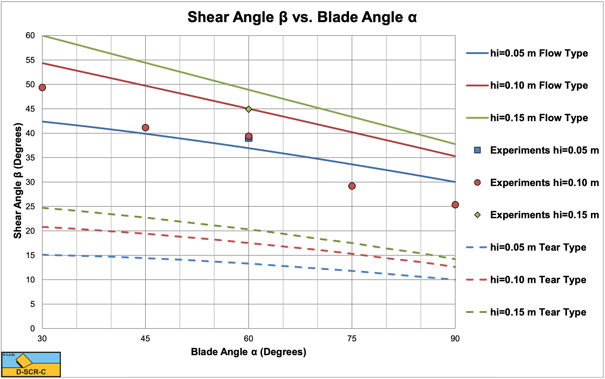
Hatamura & Chijiiwa (1977B) carried out experiments in sand, clay and loam. The experiments were carried out with blade angles α of 30°, 45°, 60°, 75° and 90°, layer thicknesses h_i of 0.05, 0.10 and 0.15 m and cutting velocities v_c of 0.05, 0.10 and 0.14 m/sec. The blade had a fixed length L₄ of 0.2 m and a fixed width w of 0.33 m. The clay/loam had a dynamic cohesion c of 27.9 kPa and a dynamic adhesion a of 13.95 kPa. Hatamura & Chijiiwa (1977B) only give the dynamic cohesion and adhesion, not the static ones. Based on equation (7-53) an average strengthening factor of about 1.5 can be determined. This factor may however vary with the blade angle and layer thickness. Hatamura & Chijiiwa (1977B) measured the shear angle β, the total cutting force and the direction of the total cutting force. The also determined the location of the acting points of the different forces. In the model they derived they used the horizontal and vertical force equilibrium equations and the equilibrium of moments equation combined with their measured acting points. By solving the 3 equilibrium equations, they solved the horizontal cutting force, the vertical cutting force and the shear angle, based on 3 equations with 3 unknowns. The theory as derived here assumes a shear angle where there is a minimum horizontal force, based on the minimum cutting energy principle. So the two approaches are different. Hatamura & Chijiiwa (1977B) found that cutting tests with cutting angles of 30° and 45° were according to the Tear Type, while the larger cutting angles followed the Flow Type of cutting mechanism. This tells something about the tensile strength of the material. Based on the above an ac ratio r of 0.5-0.7 can be derived. Figure 7-27 shows that a tensile strength to cohesion σT/c ratio of about 0.2 may explain this. So it is assumed that the tensile strength is 20% of the cohesion.

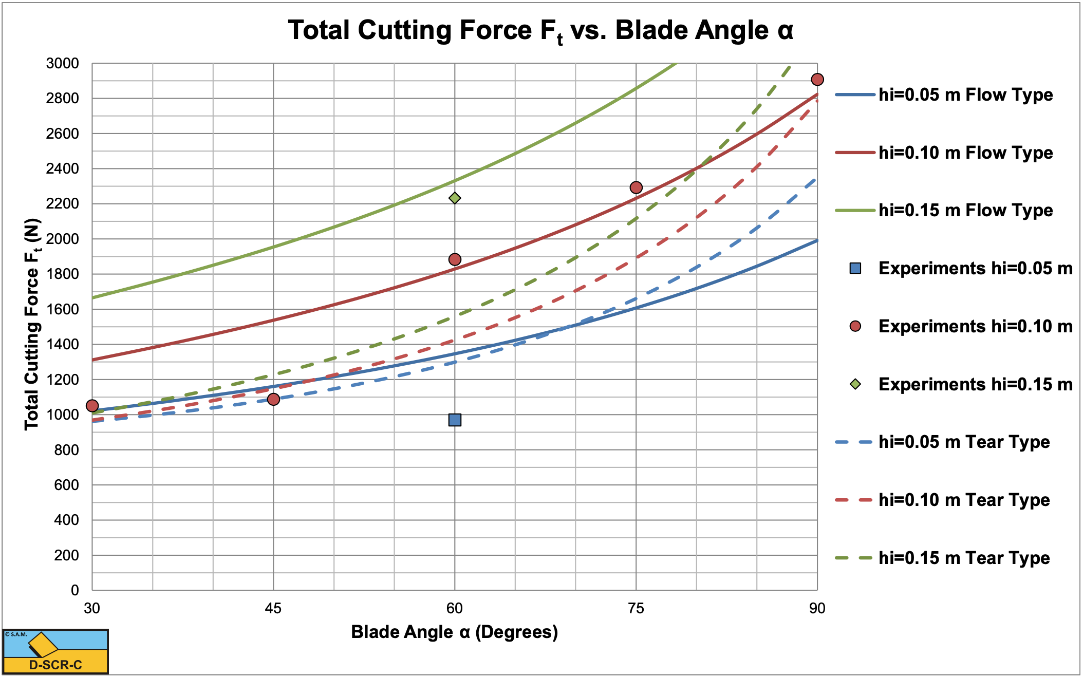
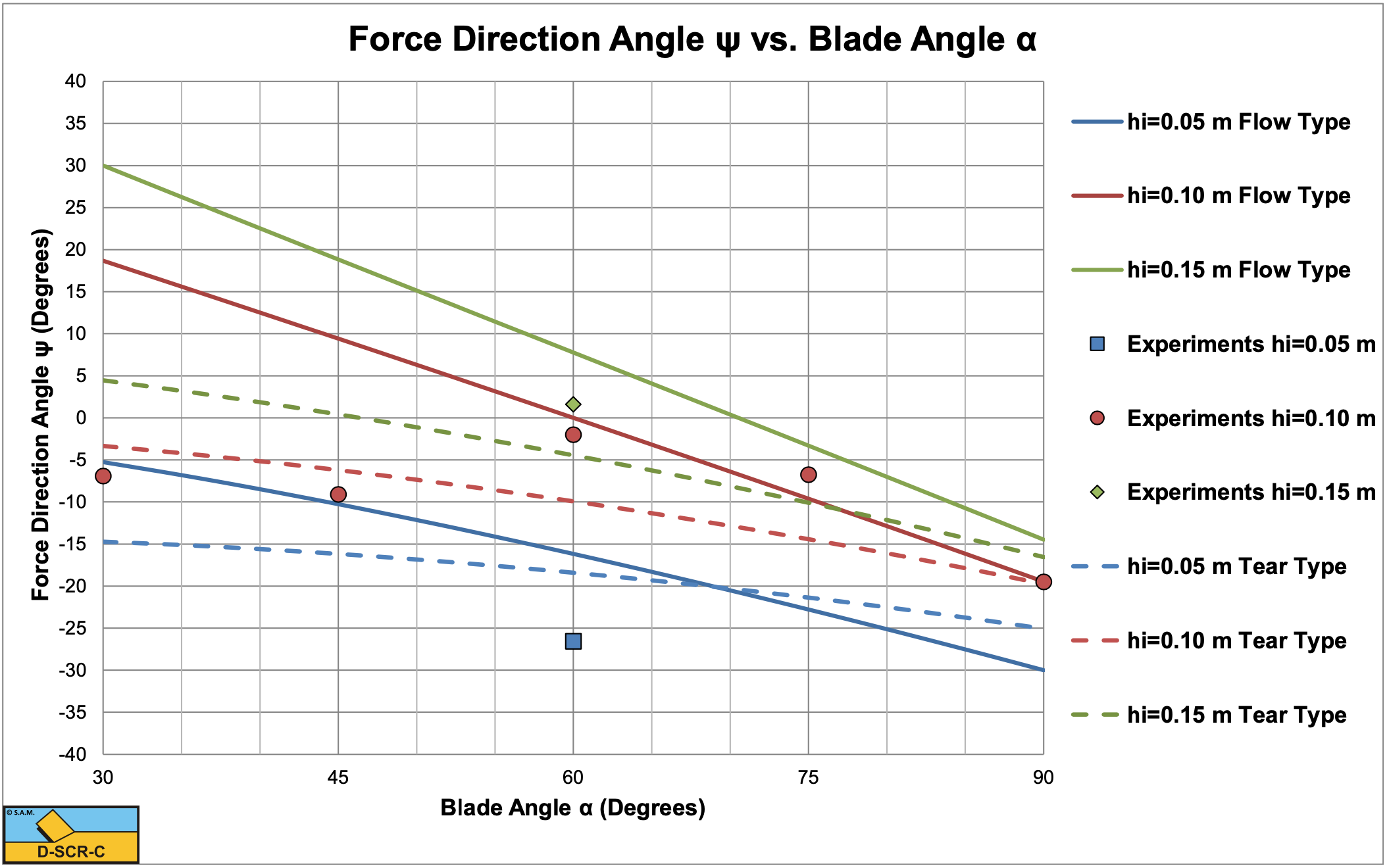
Figure 7-44, Figure 7-45 and Figure 7-46 show the results of the experiments and the calcultations. The calculations are carried out for both the Flow Type and the Tear Type. The shear angles predicted are 5°-10° larger than the ones measured, however the tendency is the same.
The measured total cutting forces match the predicted cutting forces very well for the Tear Type for blade angles of 30° and 45° and for the Flow Type for blade angles of 60°, 75° and 90°. The theory does predict the Tear Type and the Flow Type for the corresponding blade angles. The directions measured of the total cutting force also match the theory very well if the correct cutting mechanism is considered. So apparently the total cutting forces and the direction of these forces can be predicted well, but the shear angle gives differences. We should consider that the shear angle as used in the theory here is a straight line, a simplification. In reality the shear plane may be curved, leading to different values of the shear angle measured. For the Tear Type it is not clear what definition Hatamura & Chijiiwa (1977B) used to determine the shear angle. Is it the point where the secondary tensile crack reaches the surface? This explains some of the differences between the measured and calculated shear angles. Overall, the theory as developed here predicts the cutting forces and the direction of these forces very well.

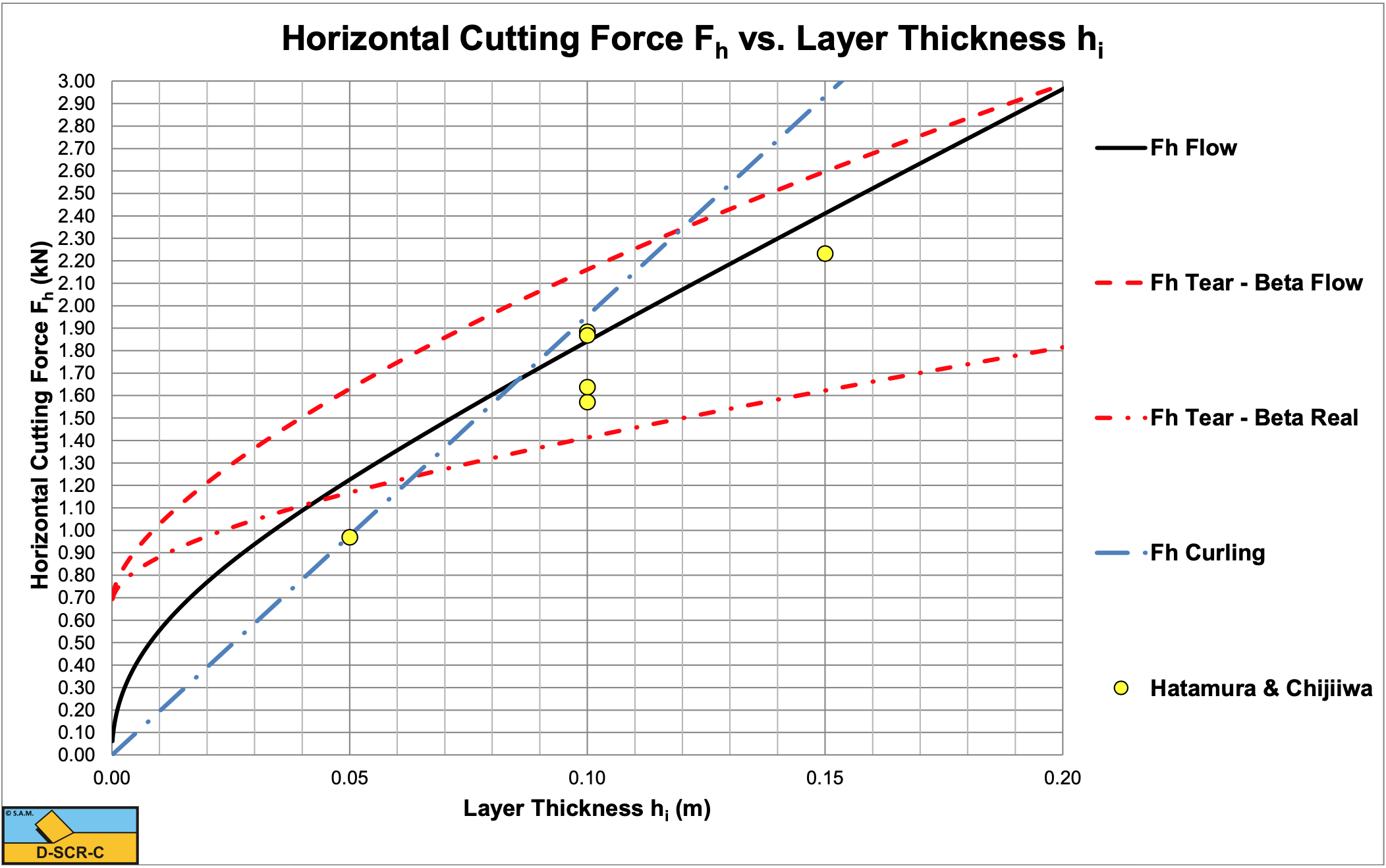
The force for a 60° blade and 0.05 m layer thickness is smaller than expected based on the Flow Type of cutting process. This is caused by the Curling Type as shown below.

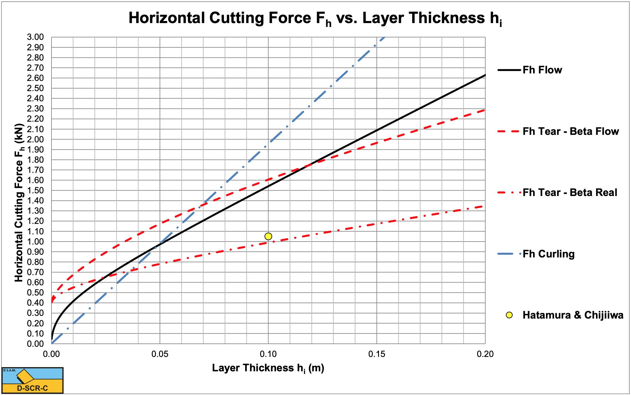
Figure 7-45 shows that the experiment with a layer thickness of 0.05 m with a blade angle of 60° gives a smaller cutting force than estimated. Analyzing the 60° experiments as a function of the layer thickness gives Figure 7-47. This figure shows that up to a layer thickness of about 0.08 m there will be a Curling Type of cutting process. Above 0.08 m there will be a Flow Type of cutting process, while above about 0.20 m there will be a Tear Type of cutting process. Once the Tear Type is present, the force will drop to the lower Tear Type curve as is visible in the 30° and 45° experiments. Since all 3 cutting mechanisms were present in the experiments of Hatamura & Chijiiwa (1977B), it is not possible to find just one equation for the cutting forces. Each of the 3 cutting mechanisms has its own model or equation. Figure 7-48 shows the 30° experiment. It is clear from the figure that at 0.10 m layer thickness the cutting mechanism of of the Tear Type.

Figure 7-44: The shear angles measured and calculated.

Figure 7-45: The total cutting force measured and calculated.

Figure 7-46: The direction of the total cutting force measured and calculated.

Figure 7-47: The 60 degree experiments.

Figure 7-48: The 30 degree experiment.

7.8.2. Wismer & Luth (1972B)

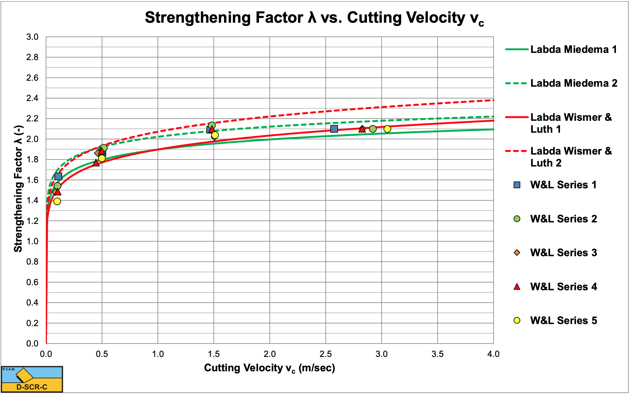
Wismer & Luth (1972B) investigated rate effects in soil cutting in dry sand, clay and loam. For clay and loam they distinguished two rate effects, the inertial forces and the strengthening effect. For cutting velocities as known in dredging (up to 5-6 m/sec), the inertial forces can be neglected compared to the static cutting forces (low cutting velocities) and compared to the strengthening effect. Wismer & Luth (1972B) carried out experiments with blade angles of 30°, 60° and 90°, blades of 0.19·0.29 m, 0.127·0.193 m and 0.0762·0.117 m (7.5·11.45 inch, 5.0·7.6 inch and 3.0·4.59 inch) and layer thicknesses from 0.0225-0.0762 m (0.9-3.0 inch). They did the experiments in two types of clay. Unfortunately they did not mention the cohesion and adhesion, but the mentioned a cone resistance. However, based on their graphs the cohesion could be deducted. The cone index 27 clay should have had a cohesion of about 22.5 kPa and an adhesion of 11.25 kPa, the cone index 42 clay a cohesion of 34 kPa and an adhesion of 17 kPa. The strengthening factor of Wismer & Luth (1972B) can be rewritten in SI Units, using the reference strain rate of 0.03/sec, giving the following equation for the strengthening factor.

\[\ \tau=\tau_{\mathrm{y}} \cdot \lambda_{\mathrm{s}} \quad\text{ with: }\quad \lambda_{\mathrm{s}}=\left(\frac{\frac{\mathrm{v}_{\mathrm{c}}}{\mathrm{h}_{\mathrm{i}}}}{\mathrm{0 . 0 3}}\right)^{\mathrm{0 . 1}}\tag{7-106}\]

Figure 7-49 shows the theoretical strengthening factors based on the average of equations (7-34) and (7-35) and for the above equation for the minimum and maximum layer thickness, giving a range for the strengthening factor and comparing the Miedema (1992) equation with the Wismer & Luth (1972B) equation. The figure also shows the results of 5 series of tests as carried out by Wismer & Luth (1972B) with a 30° blade. The two equations match well up to cutting velocities of 1.5 m/sec, but this may differ for other configurations. At high cutting velocities the Wismer & Luth (1972B) equation gives larger strengthening factors. Both equations give a good correlation with the experiments, but of course the number of experiments is limited. A realistic strengthening factor for practical cutting velocities in dredging is a factor 2. In other words, a factor of about 2 should be used to multiply the static measured cohesion, adhesion and tensile strength.

It should be mentioned that the above equation is modified compared with the original Wismer & Luth (1972B) equation. They used the ratio cutting velocity to blade width to get the correct dimension for strain rate, here the ratio cutting velocity to layer thickness is used, which seems to be more appropriate. The constant of 0.03 is the constant found from the experiments of Hatamura & Chijiiwa (1977B).

Figure 7-49: The strengthening factor.